![]()
![]()
Let's look first at the whole input file, using an example of a vertical strike-slip fault driven by dextral simple shear:
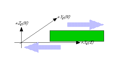
The input file is reproduced below. The important or relevant pieces are linked to text below the input file; these links provide an annotation of the input file.
* POISSONS RATIO YOUNGS MOD #PLANES COEFF INTERNAL FRICTION BACKGROUND DEFORMATION (See manual)
 .25                   7.E10      2                            0.6                           displacement gradient
* Background (blank; Exx,Exy,Exz,Eyy,Eyz,Ezz; Sxx,Sxy,Sxz,Syy,Syz,Szz; dUx/dx /dy /dz,dUy/dx /dy /dz,dUz/dx /dy /dz)
-.5e-4 .5e-4 0     -.5e-4  .5e-4 0    0 0 0

for each plane:
ORG:XO   YO   ZO                WDTH:STK  DIP  #SUB-ELEM:STK  DIP  STK    DIP
     10.0  10. 0.0                 50.   20.            3    2   45.   90
    38.2843 52.4264  0.0            50.   20.            3   2   45.   90

for each plane (at each fixed distance along strike, going up-dip):
PLN,SUB-ELEM           code    BC-shear(STK)   BC2-shear(DIP)  BC3-normal
1
     1   1       12         0.         0.0             0.0
     1   2       12         0.         0.0             0.0
     1   3       12         0.         0.0             0.0
     2   1       12         0.         0.0             0.0
     2   2       12         0.         0.0             0.0
     2   3       12         0.         0.0             0.0
2
     1   1       12         0.         0.0             0.0
     1   2       12         0.         0.0             0.0
     1   3       12         0.         0.0             0.0
     2   1       12         0.         0.0             0.0
     2   2       12         0.         0.0             0.0
     2   3       12         0.         0.0             0.0

* Run everything else interactively
Non-interactive grid specification
plane
vector
* Coordinate system of output
in-plane
* Output files to create
stress
elements
* Output file suffix
pln
* Xo, Yo, Zo (Ref.corner), strike,dip,length,width:
10.1 10.1 0.  45. 90.  50. 20.
* number of grid points in the strike and dip directions
50 20.
0 1e-4 0 0 0 0 0 0 0
is the row-by-row displacement gradient tensor, and it specifies a dextral or right-lateral simple shear.
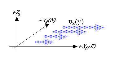
If you wanted to dimensionalize this, you might assume, as an example, that the region being deformed is 100 km across (say 50 km each side of the fault), so that a shear of 1e-04 is generated by a relative displacement of 10m. If you were modeling the San Andreas fault, for example, this would correspond to a time interval between 200 and 300 years.
Go here for other methods of driving the deformation.
ORG:XO   YO   ZO                WDTH:STK  DIP  #SUB-ELEM:STK  DIP  STK    DIP

      10.0  10.1 0.0                 100.   20.            3    2   90.   90
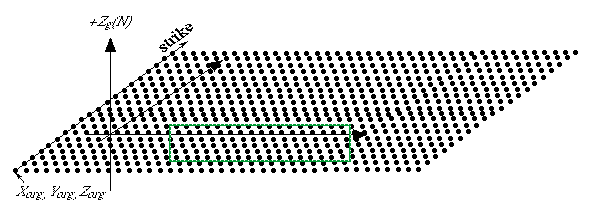
means that the top left of the plane lies 10 km east and 10.1 km north of the origin, and is at the surface. It is 100 km long, 20 km down-dip, has a subelement every ~33 km along strike and every 10 km down-dip. The plane strikes due east, the hangingwall is the southern block, and it's vertical. Like this:
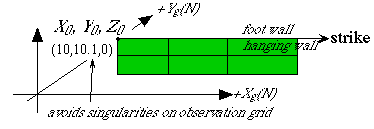
![]() It is important to offset slightly either the
fault-plane or the inspection grid (see below) from each other to avoid
the calculation of singularities at the edges of subelements.
It is important to offset slightly either the
fault-plane or the inspection grid (see below) from each other to avoid
the calculation of singularities at the edges of subelements.
Specifying boundary conditions:
1
     1   1       12         0.         0.0             0.0
     1   2       12         0.         0.0             0.0
     1   3       12         0.         0.0             0.0
     2   1       12         0.         0.0             0.0
     2   2       12         0.         0.0             0.0
     2   3       12         0.         0.0             0.0
2
     1   1       12         0.         0.0             0.0
     1   2       12         0.         0.0             0.0
     1   3       12         0.         0.0             0.0
     2   1       12         0.         0.0             0.0
     2   2       12         0.         0.0             0.0
     2   3       12         0.         0.0             0.0
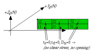
The single fault-element in this example has a total of 6 subelements, 3 along strike, 2 down-dip. The first two columns specify the identity of the subelement (col row). Remember that columns start at the left and rows start at the bottom. Thus (1,1) is at the lower left and (3,2) is at the top right.
![]() In most input files that you see from now on, the
(col row) identifiers of subelements will be 1s only, because these
numbers are not read by the program. The program expects the
subelements to be ordered properly, and the numbers are really only for
the user.
In most input files that you see from now on, the
(col row) identifiers of subelements will be 1s only, because these
numbers are not read by the program. The program expects the
subelements to be ordered properly, and the numbers are really only for
the user.
The boundary conditions shown here correspond to code 12 (strike//stress, dip//stress, normal_relative displacement) and are zero for each component. This means that the strike and dip relative displacement at the center of each subelement will be such that the final state of shear stress is zero, and that there is no normal opening or closing. Code 12 0 0 0 is a common bc for freely slipping fault-elements.
plane
xyz
* Coordinate system of output
global
* Output files to create
displacements
elements
strain
stress
* Output file suffix
out
Results are to be output to a plane in only xyz format and in global coordinates. Four types of results will be calculated, displacements on the inspection plane (see below for details of the inspection plane), displacements across each of the subelements, and components of the strain and stress tensor on the inspection plane. Result files will be identified by their suffix .out.
* Xo, Yo, Zo (Ref.corner), strike,dip,length,width:
-50 -50 0 0 0 200 200
* number of grid intervals in the strike and dip directions
50 50
The inspection plane is specified in the same way as an element. This one is horizontal and at the ground surface and is 200 km by 200 km. Each side is divided into 50 even increments, which will yield 51x51 point-calculation results. The inspection plane is defined to be well away from fault edges in order to adequately sample the subtle variations in displacement, strain, etc. away from the fault.
An example of an output file (file: elements.out) showing displacements across the subelements is shown below.

(The top header line is not usually part of the output file.)
Notice that both strike-parallel and dip-parallel relative displacements are negative, which means that the hangingwall is moving relative to the footwall along -Xp and -Yp, so that the fault is dextral and normal, although the strike-slip component is an order of magnitude larger than the normal component. And as specified in the input file boundary conditions, the fault-normal displacements are zero.
Given this type of fault, the vertical displacements should be as shown below:
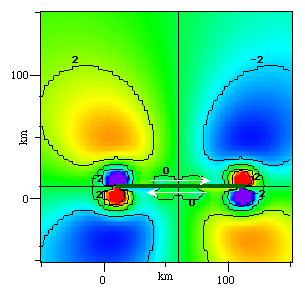
Vertical displacements (cm) must be 'up' in contractional quadrants (file displacements.out), as indeed they are here.
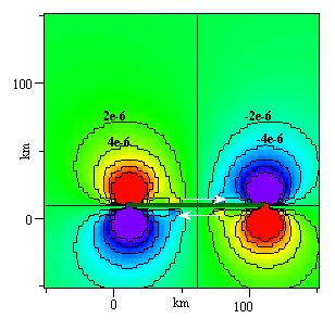
And contractional strains (negative = blues) should occupy the contractional quadrants (file strainten.out); see below.
Other examples of both input and output can be found in Examples on the main menu and in Output.