Generic Mapping Tools 4
This final GMT lab will look at plotting grid-based data on maps, which can be a bit more complicated than plotting point-based data. With the increase in availability of densely sampled, high quality geophysical datasets, knowledge of how to plot and display grid-based data in GMT is an essential skill for any geophysicist.
ASCII Data
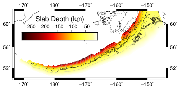
The first example uses a dataset containing ASCII data of the geometry of the Alaskan subduction zone. You will need to either copy this file from my public folder into your working directory, modify the shell script to include the full path to its location in my public folder (/gaia/home/egdaub/Public/dataanalysis/alu_slab1.0_clip.xyz), or download it from the USGS site. This is the first plot (gmt4_1.pdf) produced by the shell script (gmt4.csh):
Here are the commands (GMT 4):
xyz2grd alu_slab1.0_clip.xyz -Galaskaslab.grd -R167/216/50/62 -I0.02
grd2cpt alaskaslab.grd -Chot -Z > alaskaslab.cpt
grdimage alaskaslab.grd -Calaskaslab.cpt -R -JM5i \
    -Q -K -P > gmt4_1.ps
grdcontour alaskaslab.grd -C30 -J -R -Wdarkgray -A- -K -O -P \
    >> gmt4_1.ps
pscoast -R -J -B10/4 -W -Di -Ir -N1 -K -O -P >> gmt4_1.ps
psscale -D1.5i/1.5i/2.5i/0.25ih -Al -Calaskaslab.cpt \
    -B50:"Slab Depth (km)": -O -P >> gmt4_1.ps
and for GMT 5, this is:
gmt xyz2grd alu_slab1.0_clip.xyz -Galaskaslab.grd -R167/216/50/62 -I0.02
gmt grd2cpt alaskaslab.grd -Chot -Z > alaskaslab.cpt
gmt grdimage alaskaslab.grd -Calaskaslab.cpt -R -JM5i \
    -Q -K -P > gmt4_1.ps
gmt grdcontour alaskaslab.grd -C30 -J -R -Wdarkgray -A- -K -O -P \
    >> gmt4_1.ps
gmt pscoast -R -J -Bx10 -By4 -W -Di -Ir -N1 -K -O -P >> gmt4_1.ps
gmt psscale -D1.5i/1.5i+w2.5i/0.25i+h+jCT+m -Calaskaslab.cpt \
    -Bx50+l"Slab Depth (km)" -O -P >> gmt4_1.ps
with the commands given in the shell script being:
xyz2grd $infile -G$gridfile -R${xmin}/${xmax}/${ymin}/${ymax} -I$gridspace
grd2cpt $gridfile -C$cmap $cmapcont > $cptfile
grdimage $gridfile -C$cptfile -R -JM$size \
        $masknan $firstplot $portrait > $outfile
grdcontour $gridfile -C$contourint -J -R -W$contourcolor -A$contourlabel $midplot $portrait \
        >> $outfile
pscoast -R -J $bvals -W -D$resolution $rivers $natbounds $midplot $portrait >> $outfile
set code = "psscale $scalvals -C$cptfile $bvalscbar $finalplot $portrait >> $outfile"
eval "$code"
This plot introduces several new commands, which I describe below.
xyz2grdis a command that translates an ASCII file (or binary) containing grid-registered data into a GMT grid file. It requires the arguments given in this command, namely a file from which to read, a destination file to write the gridded data (-Galaskaslab.grd), the-Rflag to specify the extent of the data, and the-Iflag, which specifies the sampling interval of the grid (in this case, the file is sampled at 0.02 degrees). All of these arguments are required.grd2cptthen takes the grid file and sets up a color palette for plotting the data. This works in a manner similar tomakecptthat we saw in the previous lab, but uses the limits of the grid file to determine the color scale (rather than the way I manually set the limits in the example from the last lab). The command takes the grid file as an argument,-Chotspecifies the color scale, and-Zmakes the colorscale continuous. The resulting color palette file is written toalaskaslab.cpt.- Now I begin doing the actual map plotting. I would like the coastlines to act as an overlay on the subduction geometry, so I use
grdimageto display the color scaled image first.grdimagetakes several arguments, most of which should be familiar to you:- First is the grid file,
alaskaslab.grd -Calaskaslab.cptdefines the color palette used to display the data-Rspecifies the region, which is the same as the previous use of-R-JM5isets the projection-Qis a new option. For this example, we have a grid file that is defined over a region that is larger than the range of the actual data. To distinguish between data points and non-data points, the non-data points haveNaNas the entry. Each color palette has a set color that it uses to displayNaNvalues. Here, I do not want theNaNvalues to display any color, because I would like to see the map coastlines that I will plot later. The-Qoption makes theNaNvalues transparent, and they will not show up in the final image.-Ksays that more commands are to follow, and-Psets portrait mode. Output is then written to file.
- First is the grid file,
- Next, we use
grdcontourto draw contour intervals on the color image. The options forgrdcontourare as follows:- First, we give the grid file,
alaskaslab.grd -C30defines the contour interval to be 30 km. Alternatively, if you have a discrete color palette, you can call the-Coption with the cpt file and the contour intervals will be set by the color intervals in the color palette file.-J -Rare the usual projection and region options-Wdarkgraysets the pen used to draw the contour lines-A-means that I do not want the contours labeled (I will put a colorbar on the plot later to show the values)-K -O -Phave their usual meanings, and output is appended to the file
- First, we give the grid file,
pscoastdraws the coastlines. This command does not contain any new options.psscaledraws the colorbar. I have not used any new options here, so if you are unsure of this command, refer back to the notes for the previous class.
As you can see, dealing with gridded data usually involves some additional commands to set everything up before plotting the data.
Topographic Data
We might expect that there are certain types of data that are likely to be needed by all users of GMT, such as topography and bathymetry data. These types of data are often added to plots in addition to the data in question, as it makes plots look nice and makes them easier to interpret. Because these datasets are also quite large as they are often defined for the entire globe, it makes sense to have them available in one central location that is readable by GMT so that each user does not have to obtain a duplicate copy.
There are a number of such datasets available in the Mac Lab. To see what is available, type grdraster (gmt grdraster for GMT 5) into the command prompt. You will see something like this (you may need to scroll up to see this):
#   Data Description            Unit    Coverage                Spacing     Registration
-----------------------------------------------------------------------------------------
1   "ETOPO5 global topography"  "m"     -R0/359:55/-89:55/90    -I5m        GG
2   "US Elevations from USGS"   "m"     -R234/294/24/50         -I0.5m      PG
This will be followed by a number of other datasets. These are the sets available to you thanks to your friendly system administrators, who went to the trouble of finding, downloading, and setting them up for you. This tells us some of the details of each of these files. The first one is “ETOPO5 global topography” which gives the meters of elevation (negative values for bathymetry) over a grid from \({0^\circ}\) to \({359.55^\circ}\) and \({-89.55^\circ}\) to \({90^\circ}\) with a spacing of 5 minutes, and the GG means the data is grid-registered with geographic coordinates (i.e. values are given for every grid point rather than a pixel value, and the registration of the grid values in the file are in geographic, rather than cartesian order, meaning longitude varies first).
To use these files, we use the grdraster command, followed by the file number, and then the other options that are similar to xyz2cpt above and write the data to a grid file. We can then display the data using the grdimage command as it was used above.
If you want to install GMT on your own computer, then you will need to install these databases yourself, as they do not come with GMT. All of the data is freely available, so as long as you can find the datasets online, download them, and configure the grid information file, you should be able to use the following GMT commands on your own machine without any problems. However, it is even easier to just copy the files off of the Mac Lab computers and into the appropriate directory in your GMT installation. In the Mac Lab, the GMT databases live in /usr/local/GMT4.5.7/share/dbase/ (you will need to use a terminal to see them). That directory contains the databases, plus a grid information file grdraster.info that contains information about them. You need to copy any datafiles that you want to use (note: some of these files are very large, meaning you may need to bring a portable hard drive to copy them), plus the grdraster.info file to the directory /<path_to_GMT>/share/dbase/ on your own computer. (Note: I am not sure how these data files work on Windows.) You are of course free to find your own gridded data to use with GMT in this way, and as more and more high resolution geophysical data becomes available you will no doubt want to use some of it in GMT to produce maps.
Topographic Shading
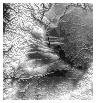
However, if we go ahead and display one of these topographic gridfiles using grdimage, we get something like this:
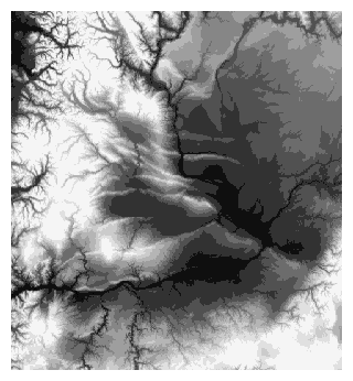
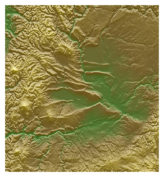
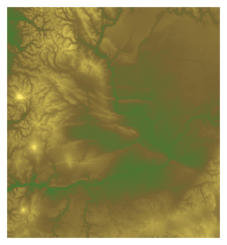
While this looks nice, it is not clear what this is topographically, since we do not have a color scale. This is because our brains are used to looking at topographic maps that are illuminated to help us interpret the topography. However, as with most things where we implicitly fill in the details, this means our brains can play tricks on us. Take the following two images of the same terrain, illuminated differently:
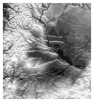
Can you tell what kind of terrain this is? It looks different on the left versus on the right, because one of them is illuminated in a way that you are not used to. The left image is illuminated from the top, while the right image is illuminated from the bottom, and usually these types of images are illuminated from the north (or an angle close to that of north).
Unfortunately, by illuminating we lose some of the quantitative information on altitude (particularly for grayscale images) even if the light and shadows help our brain interpret the image. Thus, the best option is usually to combine both color and illumination. Here is the color version of the image illuminated from the north, side by side with the non-illuminated version:
As you can see, the shading helps your brain interpret the topography, and by keeping the color scale, we can better determine which areas are high and which areas are low.
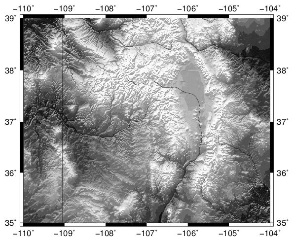
Making a Shaded Topographic Plot
How do we make shaded plots? Here is an example showing how it is done (the resulting file is gmt4_2.pdf):
And the code for this plot is as follows for GMT 4:
grdraster 11 -R-110/-104/35/39 -I0.5m -Gfctopo.grd
grd2cpt fctopo.grd -Cgray > fctopo.cpt
grdgradient fctopo.grd -A345 -Gfctopo.intns -Ne0.6
grdimage fctopo.grd -Ifctopo.intns -Cfctopo.cpt -R -JM5i \
    -K -P > gmt4_2.ps
pscoast -R -J -B1 -Dh -Na -Ir -P -O >> gmt4_2.ps
In GMT 5, the same plot is produced using:
gmt grdraster 11 -R-110/-104/35/39 -I0.5m -Gfctopo.grd
gmt grd2cpt fctopo.grd -Cgray > fctopo.cpt
gmt grdgradient fctopo.grd -A345 -Gfctopo.intns -Ne0.6
gmt grdimage fctopo.grd -Ifctopo.intns -Cfctopo.cpt -R -JM5i \
    -K -P > gmt4_2.ps
gmt pscoast -R -J -Bx1 -By1 -Dh -Na -Ir -P -O >> gmt4_2.ps
Using the variables defined in the shell script, the actual code is:
grdraster $datasetno -R${xmin}/${xmax}/${ymin}/${ymax} -I$grdinterval -G$gridfile
grd2cpt $gridfile -C$cmap > $cptfile
grdgradient $gridfile -A$intnsdirection -G$intnsfile -N$intnsnorm
grdimage $gridfile -I$intnsfile -C$cptfile -R -JM$size \
    $firstplot $portrait > $outfile
pscoast -R -J $bvals -D$resolution $natbounds $rivers $finalplot $portrait >> $outfile
These commands do the following:
grdrasterturns the data file into a grid file that GMT uses for plotting. The first argument is11, which is saying that I want to use file number 11 (ETOPO30swhich is global land topography sampled every 30 seconds – typegrdrasterwith no arguments to see the different files available). Following that, we have three required arguments:-Rto define the desired region,-I0.5mto determine the grid resolution, and-Gfctopo.grdto specify the destination grid file name.grd2cptsets the color palette to the range of values in the data. Its use is the same as above (save for a few options that I chose not to use this time).grdgradientis used to calculate the gradient of a grid in a particular direction, and one of its uses is to calculate the intensities for the topographic illumination. It takes a grid file as its input, and the-A345option selects the direction in which to take the gradient (relative to degrees north, clockwise positive). Here I pick an angle \({15^\circ}\) from north (\({345^\circ}\)).-Gfctopo.intnssets the output intensity file (really just a grid file, but I like to use.intnsto remind me that the file is normalized for adding illumination).The final option is
-Ne0.6, which tells GMT how to normalize the calculated gradient. If I wanted the true gradient, then I would not call this option. For doing illumination, we need the gradient to be in the range \({(-1,1)}\), as it determines how much to lighten or darken the colors relative to their color value. The option-Ne0.6says to normalize the gradient such that the maximum value is \({\pm0.6}\), and to have the intensities follow a cumulative Laplace distribution. There are additional distributions and parameters that you can use when callinggrdgradient(I have found this option produces plots that look nice, but feel free to try different distributions or parameters if you would like a different effect).grdimageplots the grid file. As before, we give it a color palette (-C), and region and projection information (-R -JM5i). The intensity for illumination is specified by-Ifctopo.intns.-K -Phave their usual meaning.The final command is
pscoastto draw the international and national borders, plus I color the rivers blue. Output is appended to the filegmt4_2.ps.
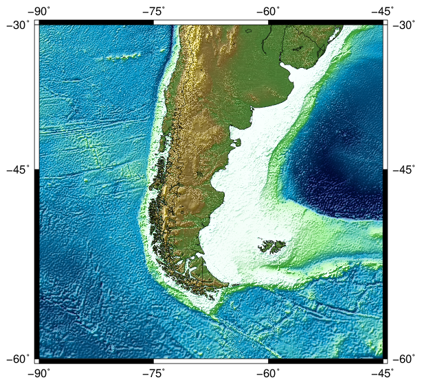
Merging Datasets
What if the last map had included an ocean area? The ETOPO30s dataset only covers continental areas, but what if we wanted to show an oceanic area’s bathymetry? GMT contains tools to combine and merge datasets, which allows you to show high resolution topography on land and lower resolution bathymetry in the oceans on the same plot. While you can do this using transparency, the best way to do this is to merge the two datasets. This allows you to produce plots showing both topography and bathymetry (gmt4_3.pdf):
The code to create this plot includes the following commands (GMT 4):
grdraster 11 -R-90/-45/-60/-30 -I0.5m -Gpattopo.grd
grdraster 10 -R -I2m -Gpatbath.grd
grdsample patbath.grd -I0.5m -Gpatbathinterp.grd
grdmath pattopo.grd patbathinterp.grd AND = pattopobath.grd
makecpt -Crelief -Z > pattopo.cpt
grdgradient pattopobath.grd -A330 -Gpattopo.intns -Ne0.6
grdimage pattopobath.grd -Ipattopo.intns -Cpattopo.cpt -R \
    -JM5i -K -P > gmt4_3.ps
pscoast -R -B15 -J -W -N1 -O -P >> gmt4_3.ps
For GMT 5, the commands are:
gmt grdraster 11 -R-90/-45/-60/-30 -I0.5m -Gpattopo.grd
gmt grdraster 10 -R -I2m -Gpatbath.grd
gmt grdsample patbath.grd -I0.5m -Gpatbathinterp.grd
gmt grdmath pattopo.grd patbathinterp.grd AND = pattopobath.grd
gmt makecpt -Crelief -Z > pattopo.cpt
gmt grdgradient pattopobath.grd -A330 -Gpattopo.intns -Ne0.6
gmt grdimage pattopobath.grd -Ipattopo.intns -Cpattopo.cpt -R \
    -JM5i -K -P > gmt4_3.ps
gmt pscoast -R -Bx15 -By15 -J -W -N1 -O -P >> gmt4_3.ps
Within the shell script, this is called as:
grdraster $topofileno -R${xmin}/${xmax}/${ymin}/${ymax} -I$topogrdinterval -G$topofile
grdraster $bathfileno -R -I$bathgrdinterval -G$bathfile
grdsample $bathfile -I$topogrdinterval -G$bathfileinterp
grdmath $topofile $bathfileinterp AND = $mergedfile
makecpt -C$cmap $cmapcont > $cptfile
grdgradient $mergedfile -A$intnsdirection -G$intnsfile -N$intnsnorm
grdimage $mergedfile -I$intnsfile -C$cptfile -R \
    -JM$size $firstplot $portrait > $outfile
pscoast -R $bvals -J -W $natbounds $finalplot $portrait >> $outfile
Here are the details on these commands:
The first two commands call
grdrasteras above. The first call togrdrasteruses the same land-basedETOPO30sdataset that we used above, which is sampled at 30 second intervals. The second call togrdrasteruses dataset 10, which is a global 2 minute sampling rate topography/bathymetry dataset (typegrdrasterfor more information on this dataset). We choose the same region for both, and sample both datasets at their full resolution (to sample the data at a lower rate, you can change the sampling rate on the-Ioption).The two grid files need to be merged, but first we must fix the fact that they are sampled at a different rate. This is done using
grdsample, which resamples a dataset to the desired grid spacing. We choose to resample the bathymetry dataset to match the higher resolution of the land topography dataset. The sampling interval is set by the flag-I0.5mto 30 seconds so that the data sampling rate matches between the two datasets.If the new sampling rate is chosen to be higher than the previous sampling rate,
grdsampleinterpolates. If the new sampling rate is more coarse than the existing data, it desamples the data (i.e. it simply takes every \({n}\)th point, without applying an anti-aliasing filter, so take care when desampling data that varies at a high rate).The next command merges the two datasets using the
grdmathcommand.grdmathdoes mathematical operations on datasets, using what is known as Reverse Polish Notation, or RPN. RPN puts the operator after the operands, using what is known as a “stack” to hold results. When using an unary operator, the operation is applied to the first item in the stack, and leaves the result in the first position on the stack. When using a binary operatory, the operation is applied to the first two items in the stack, and leaves the result in the first position on the stack (if there were any items higher up in the stack, they are shifted down a position). Array math is done element-by element (i.e. you cannot do matrix multiplication usinggrdmath, only element-by-element array multiplication).For example, if you have one grid file that you would like to take the additive inverse of (the
NEGoperator), then you would enter the following:grdmath a.grd NEG = b.grd
This would write the additive inverse of the data in
a.grdto the grid fileb.grd.To add two grid files, use theADDoperator and put the two grid files on the stack:grdmath a.grd b.grd ADD = c.grd
This will write the sum of the two grids to a third grid file. For our case, we need to use the
ANDoperator.ANDis a binary operator, which keeps the result in the first grid file, unless that file contains aNaN, in which case the operation keeps the result in the second grid file. Because all of the oceanic areas areNaNentries in ourETOPO30sdata, we can replace theNaNson the oceans with the bathymetry data from the second dataset. Thus, the resulting command is:grdmath pattopo.grd patbathinterp.grd AND = pattopobath.grd
The result is written to the file
pattopobath.grd, which we then use to plot our data.makecptcreates the color palette for displaying the data. I set-Creliefto use the “relief” color palette, and since it is already scaled for use with topography and bathymetry, I use it as is without modifying the limits. My only change is to make it continuous using-Z.grdgradientcalculates the gradient and normalizes so that we can use the intensities to illuminate our plot. The options are the same as above.Next, we use
grdimageto plot the topographic data on our map. The command syntax is discussed above, and does not use anything new.Finally, we draw the coastlines and boundaries. There is nothing new here, either.
The end result is a map showing both topography and bathymetry. You can also illuminate and shade the bathymetry and topography from slightly different directions, then merge the two instensity datasets in a similar fashion as the grid merging example above. This will make the final file look a little bit different, though I think the example above with a single illumination direction is just fine and do not see the need to go to extra trouble.
Miscellaneous GMT
Setting GMT Defaults and Parameters
GMT lets you specify absolutely any detail that you wish for your plots. As you have seen, there are many details that you specify with various command options. However, there are even more details, such as default line styles, default font names and sizes, default tick mark lengths, and on and on and on. There are several ways to set these parameters.
If you recall back to our labs on MATLAB, there were two commands to query and specify the style of plots: get and set. get allowed you to see the value of a particular option, while set allowed you to change a particular option. GMT has a similar syntax for querying and setting parameter values, using the commands gmtget and gmtset. These work in much the same way as the equivalent MATLAB commands. For a list of options, enter gmtdefaults into the terminal, or see the manual page for gmt.conf.
Alternatively, you can save default GMT values a file called gmt.conf in your working directory, home directory, or in the ~/.gmt/ directory that contains configuration options for GMT. If you do not have a gmt.conf file in your current directory, you can create one by typing gmtset -D into the terminal, or by setting a parameter value. The one in the current working directory always takes precedence, so you may want to keep a set of defaults in your home directory, but override the defaults in a working directory for a particular project.
Converting PostScript to Other Formats
Once you have created a nice GMT map, you may need to save it to a different format for use in a paper or presentation. While the Preview application on the Mac is able to do this, you can also convert formats on the command line using the psconvert command that is included with GMT. We have in fact been using this to convert files to PDF in all of the shell scripts, so this isn’t the first time we have come across this command, but here I provide a bit more detail of what it does. psconvert uses Ghostscript to convert between file formats. An example usage to convert a PostScript file to PDF would be:
psconvert -A0.1i -Tf gmt4_1.ps
The flag -A0.1i means to crop the file with a border of 0.1 inch (leaving the border size blank crops it using a tight bounding box, I usually like to add a bit of a cushion and find 0.1 inches is a good number), and -Tf sets the output format to PDF. For other output formats (there are several), see the manual. If you are converting to a raster format like PNG or TIFF, the -E option lets you specify a resolution; -E300 will save as 300 dpi.
Exercises
If you understand how all of these examples work, you will have a nice base of GMT scripts to use to create maps with data for yourself. There are also many, many examples that others have freely shared on the web, so take advantage of them. To get comfortable changing these examples, come up with your own tweaks, or try some of these.
- Change the projection.
- Change the annotations and grid lines.
- Change the color palette.
- Change the illumination direction.
- Try a different built-in dataset (type
grdrasterto get more information on them). - Change the options on the color scale (continuous vs. discrete, invert the color scale etc.). If you want to set the limits yourself, use
makecptwith the-Toption (see the previous lab). - Change the grid resolution either using
grdsampleto resample the data or by using the-Ioption when callinggrdraster. - Change the region for one of the topography plots.