It is a fundamental principle that in order to understand something, we must first know what it looks like. The shapes of sedimentary basins are critical to any understanding of the tectonic and erosional history of mountain belts, to the understanding of active vs. passive subsidence of basin floors, and to the understanding of resonance properties of the basin fill.
We are developing a promising technique that allows the shape of sedimentary basins to be determined at a relatively high resolution from ambient ground vibrations. This technique will provide a cost-effective method of characterizing sedimentary basins allowing more effective targeting of expensive reflection experiments at a later date.
We propose to apply the technique first to the northern Mississippi Embayment. We have accumulated a large number of observations that clearly show strong, stable signals in the ambient motions, that are well correlated with physical parameters of the basin.
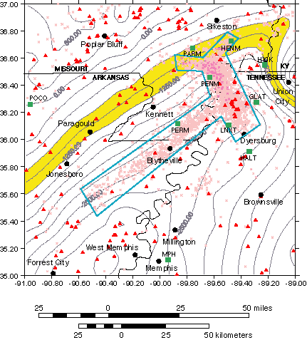
The Mississippi Embayment has a fairly simple shape (fig. 1), and its physical properties are reasonably well characterized. This facilitates numerical modeling and the interpretation of the observations. Indeed we already have a hint that forward modeling will be fruitful. We intend to rigorously test our ability to forward model the observations, and then to investigate the potential to reverse the process determining the basin shape and physical properties assuming they were not known beforehand.
The results of the proposed research will in addition become the foundation for a detailed study of basin resonances in the embayment, an important part of seismic hazard mitigation in this region. The embayment is a natural laboratory for the investigation of localized resonance and its potential effects on buildings and other sensitive structures. We have collected a rich data set on the seismic response of the embayment, and request funding to proceed to the detailed interpretation of these data.
Figure 1 is a contour map of the hard-rock surface (Paleozoic) underlying the Mississippi Embayment showing the location of broadband (BB) seismic stations currently deployed. Contours are relative to sea level, and the contour interval is 250 ft. Triangles indicate wells that sample the Paleozoic. The (light gray) crosses indicate epicenters of earthquakes recorded in the area since 1976, and the (dark gray) line outlines the New Madrid Seismic Zone. POCO (hard rock) is not a permanent station, but will continue to operate for an indeterminate time. The broadband sensors are Guralp CGM40-T that have a response flat to input velocity from 0.033 to 50 Hz. We intend to place a bore hole seismometer at Paleozoic depths near the intersection of the shaded contours with the seismic zone on another project.
THE BASIN
The Mississippi Embayment is a southwest plunging synclinal trough with a base of Paleozoic rocks (fig. 1). S-wave velocities of the rock range from 3.0 km/s (measured at the surface at Pickwick Lake, TN (Rob Williams, USGS, personal communication)) to around 3.56 km/s (Chiu, et. al., 1992). The trough is filled with generally unconsolidated sediments of Cretaceous and younger age that gently dip towards the central axis (fig. 2). The P-wave velocity, 1800m/s, is constrained through reflection profiles. Published estimates of the average S-wave velocity through the stack of sediments range from 0.6 km/s (Pujol, et al., 1996) to 0.83 km/s (Bodin and Horton, 1999). There is reasonable evidence that the average S-wave velocity increases with sediment thickness (see fig. 7B), accounting for this range of velocity estimates.
Figure 2 E-W geologic cross-section of the Mississippi Embayment at the latitude of Memphis, TN (from Bodin and Horton, 1999).
At the latitude of Memphis, TN, (fig. 2) clastic deposition has dominated since the Cretaceous. The sediment is composed largely of sand, with silt (smaller grain size) and gravel (larger) intermixed. Cycles of depositional environment have produced a layered lithology where (sand and sand-gravel) aquifers are overlain by (silty) confining units throughout the sediment column. While this layered character of the sediments is critical to ground-water flow, seismic wavelengths (of concern to seismic hazard or this study) will be large enough to average the small-scale properties of a given lithologic unit. From field investigations and the masters thesis work of Kevin Smith at CERI, we suggest that the average properties of the Eocene and Cretaceous units are quite similar while the Paleocene unit tends to smaller grain size. Initially, the sediment layer will be modeled using a depth dependent S-wave velocity structure (e.g. Vs(z)=250 h **.18 m/s, Herrmann, webpage) and constant P-wave velocity (e.g. Vp=1800 m/s).
OBSERVATIONS AND MODEL APPROACH
The first observation is that the spectral shape of ambient ground motion is different in the Mississippi Embayment than it is at a rock site adjacent to it. This is shown in figure 3 by comparing Fourier amplitude spectra from MEM (soil) and PCK (rock) in fig. 2. In general, both "noise" sources and wave propagation can contribute to the spectral shape of the ambient ground motion. We seek to discern which features in the spectral shapes (in fig. 3) are related to source differences, and which are related to differences in wave propagation. Assuming sources may have local (microtremor) or regional extent (microseisms), it would seem reasonable that local "microtremor" sources are likely to produce significant spatial variability at high frequency, while regional "microseism" sources (because they affect large areas) are likely to promote spatial similarity at long period. We have monitored the Memphis site (MEM) over time, and have noted that local trains (approximately 1 km from site) affect the amplitude spectra above frequencies of around 0.5 Hz, but do not affect the spectra below that. This leads us to suggest that the division between local and regional sources at this site occurs around 0.5Hz. This, along with observations presented later, leads us to suggest that the difference in spectral shape, observed between 0.1Hz and 0.4Hz, is likely due to differences in wave propagation at the two sites. Resonance in the soil column is our preferred explanation.
The second observation is that the spectral shape of the ambient motion is spatially dependent within the embayment. Figure 4 shows Fourier spectra of the north component of the ambient ground motion at several sites (see fig.1) for the same time period. Inspecting individual spectra reveals that the "resonance" is generally composed of multiple peaks (with the possible exception of MPH). At each site, the spectrum shows an increase in amplitude above around 0.1 Hz, and each site has a peak at around 0.22 Hz. With decreasing sediment thickness, the amplitude of the 0.22 Hz peak decreases and the frequency of the "dominant" peak increases. In the center of the basin (MPH), the resonance is relatively focused around 0.22 Hz and has large amplitude. Near the edge of the basin (PARM), the resonance is distributed in multiple peaks with lower amplitude over a broader frequency range. There is a progression in between. We suggest these spectral shapes reflect the 3D modal behavior of the basin.
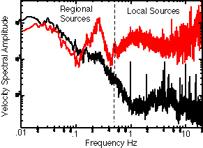
Figure 3. Comparison of ambient ground motion spectra (horizontal component) for deep soil sites (gray) and rock site (black). These observations are from the same time period. The spikes at 1Hz, 2Hz, etc. are instrumental.
Figure 5 illustrates a numerical experiment (using Finite Element codes) that shows how the SH spectrum of a resonating elliptical 2D basin is recorded at different locations over its surface (cf. Rial and Ling, 1992). The idea is that all stations record the same spectrum but with different amplitudes (shapes) depending on location. The amplitudes of the peaks are modulated by the geometry of the basin. In addition, at each station one can compute the expected 1D resonant frequency corresponding to the local sediment thickness (see fig. 5). The 1D resonant frequency computed from the local depth turns out to be a weighted-average frequency that represents (or is close to) the strongest spectral peaks excited at that locality.
This is entirely consistent with the data in fig. 4 now plotted as gray lines in fig. 5 over the predicted resonant peaks. At MPH, in the middle of the basin, the vertical fundamental predominates. As we approach the basin boundaries, the spectrum widens as higher frequency peaks (horizontal modes) grow high relative to the fundamental. We can see a number of (what we interpret to be) horizontal modes at 0.25Hz, 0.28Hz and 0.33Hz in the locality LNXT. These are all less than the expected first vertical overtone, which should be around 0.675Hz.
Figure 4. Spectral amplitudes of ambient ground motion observed at 4 BB sites (see fig.1) in the Mississippi Embayment during the same time period. The arrows indicate the location of peaks in the H/V ratio (Tp) at these sites.
Figure 5 also suggests that we can expect to refine our knowledge of the
embayment's topography/geometry or seismic velocity structure by combining observations and modeling. The approximate formulas in Rial and Ling (1992) may also be useful in the preliminary detection of the basin's structure. For a detailed analyses of the data and inversion however, the numerical approach is indispensable. To guarantee reliability in the results, numerical modeling of the embayments's seismic response will be accomplished using two independent full wave numerical solvers: GeoFlex, which is a finite element code developed by Weidlinger Associates (www.wai.com) and ELAS, a finite difference, 3D wave propagation solver developed by Shawn Larson (Lawrence Livermore Laboratory).
Figure 5 shows numerical estimates of SH-wave
spectral amplitudes at different locations on a resonant basin simulating
a 2D section of the Mississippi Embayment. The 2D basin is elliptical (1:3)
and the lower boundary is rigid. No attenuation is included. Sediment shear
wave velocity is uniform and equal to 834 m/s. Maximum depth at the center
of the basin is 960 m. On the right the f values are the approximate resonant
frequency at each place calculated by 1D formula. On the left, the maximum
spectral amplitudes on each spectrum are given in dimensionless units.
The spectra (gray) from fig. 4 are shown only to suggest the observations
may be compared to model predictions.
Our initial interest in ambient ground motion was to determine a peak in the horizontal to vertical (H/V) ratio. This peak is generally accepted to provide a measure of fundamental resonance in (shallow) soil columns for engineering application (e.g. Nakamura, 1989; Lermo and Chavez-Garcia, 1993; Field et al., 1995). Numerical simulations (Field and Jacob, 1993; Lachet and Bard, 1994) find that (in 1D models) wave propagation (dominately Rayleigh waves) from non-coherent sources is organized by geologic structure, so that the H/V ratio peak is close to the fundamental resonance mode of vertically propagating S-waves in a sediment layer. Seht and Wohlenberg (1999) and Bodin and Horton (1999) observe a correlation between the dominate peak in the H/V ratio and sediment thickness overlying Paleozoic rock in the Rhine Embayment (Germany) and the Mississippi Embayment, respectively.
Figure 6 shows observed H/V spectral peaks for an E-W line roughly corresponding to the cross section (MEM to BHP) in fig. 2. Three peaks are generally observed at any location, and the trends in space suggest that a commonality for each period range. Tl has been correlated with the thickness of the Loess blanket covering Shelby County. Tm may be partly a harmonic of Tp, and a fundamental resonance in the top 120m of sediment (modified from Smith, master's thesis).
A large number of these (H/V ratio) observations have now been made throughout the Mississippi Embayment. In general at a given site, three frequency ranges have larger horizontal than vertical motion. This gives rise to three generalized peaks in the H/V ratio (fig. 6), called here Tp, Tm and Tl . Tp and sediment thickness above the hard rock (fig. 7A) are strongly correlated, and Tl is correlated with near surface lithology (Smith, master's thesis). Tm is more enigmatic (see figure caption). The identification of three peaks in the H/V ratio is not typical in other studies, much less the correlation of two peaks with the local geology. This unique data set promises to greatly increase the utility of a commonly used, if not well understood, technique (the H/V ratio of ambient ground motion).
Figure 7A shows Tp plotted against sediment thickness overlying hard rock. The linear fit to the data has a large correlation coefficient (0.94), and a standard deviation of 0.23 s. The correlation between Tp and sediment thickness is a strong indicator that ambient ground motion can be used to infer basin geometry. Given an estimate of Tp, the thickness of the sediments underlying the observation site can be predicted to within plus or minus 80 m with 95% confidence, on the basis of this correlation (2 < Tp < 5 s). This does not require a physical interpretation of the H/V ratio. To the extent that this correlation applies to other basins, it is a useful first order predictor of basin geometry. In fig. 7B, we added the observations of Seht and Wohlenberg (1999) from the Rhine Embayment to ours. Both data sets agree for sediment thickness between 200 and 600m. Figure 7B also shows that a linear prediction equation is not adequate from 0 to 200 m.
However a physical interpretation is desirable. If we interpret Tp as the fundamental shear-wave resonance in the sediment layer, then Tp is equal to the four-way, S-wave travel time in the layer (Tp=4(h/V)). We can then estimate VTp, the average shear velocity in the sediments at each site (fig. 7C). This estimate can be compared to Vsp, the average shear velocity estimated from the delay between S-wave arrivals and S to P conversions at the sediment/rock interface for local earthquake signals (ts-tsp = h(1/vs-1/vp)). In general, VTp is slightly larger than Vsp, and both estimates indicate that the average velocity increases with sediment thickness. Field and Jacob (1993) observe a 10% shift to longer period in the peak of the H/V ratio with respect to the fundamental resonance period based on a 1D numerical model. In fig. 7 D, we shift our Tp observations to longer period by 10%, and the agreement between VTp and Vsp is improved. Two things are important: 1) Tp is sensitive to velocity structure, suggesting that we can infer velocity structure from the observations, and 2) interpreting Tp as the fundamental shear-wave resonance in the sediment layer appears to overestimate VTp by about 10%. We need to model the data to insure the correct interpretation.
Figure 7 A) The fundamental peak in the H/V ratio of ambient ground motion is plotted against sediment thickness. The linear fit (with plus or minus 2s) is also shown. B) Data from Seht and Wohlenberg (gray triangles) are included (Note scale change). C) We plot two independent estimates of the average S-wave velocity as a function of sediment thickness (see text). D) Tp values are increased by 10% (Field and Jacob, 1993) before calculating velocity.
We observe from fig. 4 that Tp is not readily identifiable within the broad resonance shape in the horizontal spectrum at some sites. This suggests the vertical spectrum plays a role in the H/V ratio, perhaps other than the commonly assumed role of removing source effects. Figure 8 shows the Fourier Spectra of the vertical components corresponding to the horizontals in fig. 4. At LNX T and HICK, the H/V peak actually corresponds to a hole in the vertical spectrum, as well as, a peak in the horizontal. At PARM, the peak in the horizontal component at around 0.22 Hz is minimized by a high at those frequencies on the vertical. The H/V ratio at MPH is less clearly affected by the vertical.
For this study it is important to understand why the H/V ratio works, and how it should be interpreted. The answer can also significantly impact the area of seismic hazard mitigation given the wide spread use of the H/V ratio to predict site resonance. The Vp/Vs ratio (or Poisson's ratio) may be a critical factor. We ran synthetic impulse responses (propagator matrix, Kennett and Kerry, 1979) for a single-flat layer over a half space. Holding vs=1.0 km/s and thickness of layer to 1 km, we modified Vp in the "sediment layer." In Figure 9A, Vp=1.73km/s, reflecting a Poisson's ratio of .25. Note, the resonance peak on the horizontal is about .22 Hz, and the first local minimum in the vertical spectra is around 0.7 Hz. Changing the surface layer so that Vs=2.85, to
Figure 8. Vertical component spectral amplitudes of ambient ground motion observed at 4 BB sites in fig.4. The arrows indicate the location of peaks in the H/V ratio (Tp) at these sites.
reflect a Poisson's ratio about .45, gives the spectra in fig 9B. Note the hole in the vertical component at the frequency of the fundamental resonance peak on the horizontals (0.22Hz). This hole would help create a peak at this frequency in the H/V ratio. We have repeated this experiment using a 1D wave number integration technique (Apsel and Luco, 1983) with an applied near-surface source. This source produces synthetics dominated by Rayleigh waves. Holes in the vertical spectra can be introduced for large Poisson's ratio, but the frequency at which the hole occurs is distance dependent. Lachet and Bard (1994) suggest that the peak in the H/V ratio is mainly controlled by the polarization curve of fundamental mode Raleigh waves, which in turn exhibit a sharp peak around the fundamental resonance mode of the sedimentary structure. They also suggest that the amplitude of the peak is highly sensitive to Poisson's ratio.
We have made limited H/V spectral ratio observations in several basins in the western US, to get a feel for the range of basin types for which the method might work. The only two that didn't show a positive result, Dixie Valley and Railroad Valley, are both in central Nevada and both are extremely dry. Dry sediments could have a low Poisson's ratio. These basins are also deep and narrow which can also be a limiting factor. 2D numerical modeling can be used to test the limitations.
SUMMARY
The distinction between signal and noise is that signal can be interpreted. We have shown a number of observations that indicate there are signals in the ambient ground motion. While the interpretation needs refinement, we are well on the way. 1D numerical models (Field an Jacob, 1993; Lachet and Bard, 1994) have shown good success at predicting the H/V ratio period. We propose to extend this modeling to 2D and fit the results to our observations. This is the logical next step.
The work we propose is:
Figure 9 shows the synthetic impulse response for a single-flat layer over a half space. The hole in the vertical component at the frequency of the fundamental resonance peak on the horizontals (0.22Hz) is produced for large Vp/Vs. This hole would help create a peak at this frequency in the H/V ratio.