*The
information presented on this web page is preliminary and should not be
used for any official or unofficial purposes.*
The Memphis, Shelby County, Tennessee, Seismic Hazard Maps
 Downtown Memphis, the Mississippi
River, and Arkansas.
|
This documentation provides an overview of how we made the Memphis seismic hazard maps. These maps complement the USGS national seismic hazard maps, which do not include the effects of local geologic structure. However, we emphasize that the Memphis maps are still regional in nature and should not be used in place of site specific studies. |
| In Memphis, Shelby
County, Tennessee damaging earthquakes are only moderately likely, but
the consequences of earthquakes, from the New Madrid seismic zone, are
likely to be very high. This densely populated urban area is built on a 1-kilometer-thick (0.62 miles) sequence of soils, sands, clays and other sediments deposited in a trough known as the Mississippi embayment; geographically the embayment approximately underlies the Mississippi Valley. This thick pile of sediments significantly changes the way the ground shakes during earthquakes. 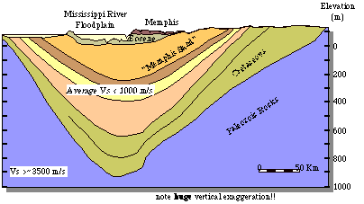 Since 1998, the U.S. Geological Survey (USGS) and its partners have been working to produce earthquake (seismic) hazard maps that account for the effects of the sediments. |
|
| Like the national maps,
the Memphis maps are 'probabilistic'. This means that the hazard is
expressed in terms of the levels of ground shaking that have a
specified chance of being exceeded in a given time period. For
example, a '2% probability of exceedance in 50 years' map shows the
levels of ground shaking that have a
1-in-50 (i.e. a 2%) chance of being exceeded in a 50 year period.
The choice of which map to use depends upon the needs of the
user. Builders of a dam, for instance, might want to consider a lower
likelihood that shaking will be exceeded (e.g. maybe 2% in 50
years) than a home builder (e.g. maybe 10% in 50 years).
This is because damage to the dam would have a greater impact on
society. |
|
 |
 |
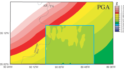
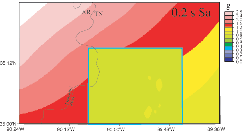
| Probabilistic
hazard maps showing ground motions with a 2% (left) and 10% (right) probability
of exceedance in 50 years. Inset map of
Memphis, Shelby County includes effects of sediments, superimposed on
the larger national seismic hazard map that does not. Before summarizing what probabilistic ground motions mean and how they're calculated, first note that although the maps show ground motions as continuously varying colors, the ground motions are actually calculated on a grid of points covering the mapped area. Thus, we can consider how the ground motion is estimated at one location on the map, as the same process is repeated at all other points. Probabilistic maps allow us to incorporate all available information about the rate at which earthquakes occur in different areas and on different faults, and on how far strong shaking extends from all likely earthquake sources. This is desirable because there may be multiple ideas about how to characterize these processes, and because we want to include the variability we know exists in nature and that arises from unavoidable measurement inaccuracy. To incorporate this range of ideas and variability, many estimates of ground motion are calculated for different combinations of input parameters. The average of these estimates is found, with those estimates derived from more accurately known parameters given more weight in the averaging. This average ground motion estimate represents the 'best' estimate statistically and is what is plotted on the map. Thus, importantly, the maps do NOT display the worst case ground motions. The probabilistic nature of these ground motion estimates can be understood in several different ways. Because ground motions come from earthquakes that occur a different rates, the estimated ground motions they cause will differ depending on the time period - or equivalently the probability level - considered. For a given time period and a LARGE probability level, the map will show the relatively likely ground motions, which are LOW because small magnitude earthquakes are much more likely to occur than are large magnitude earthquakes. For a SMALL probability level, the map will emphasize the effect of less likely earthquakes: larger magnitude and/or closer distance events, producing overall LARGE ground motions on the map. Another way to think about probabilities is to consider recurrence or repeat times. For example, an annual probability of 1% of some 'event' is equivalent to an occurrence once every 100 years, an annual probability of 10% to a recurrence time of 1000 years, etc. If instead of using an annual or 1-year interval one considers a 50-year interval; then a 10% probability would correspond to a recurrence time of 500 years (50 divided by .1), 2% to 2500 years, etc. It is important to remember that in this context the recurrence or repeat time refers to how often one expects the ground motions shown to be exceeded, NOT to how often of a particular magnitude earthquake is expected to occur. Our maps display the hazard for 2%, 5%, or 10% probabilities of exceedance in 50 years. In terms of repeat times, these tell us that we should expect the ground motions shown on these 2%, 5%, or 10% maps to be exceeded once every 2500, 1000, or 500 years, respectively. Again, these refer to ground motions, and should not be confused with the repeat times of major earthquakes in the New Madrid seismic zone of approximately 500 years. Probabilistic maps differ from more familiar 'scenario' maps that show the shaking expected for a single earthquake and one set of input parameters, regardless of the likelihood or accuracy of any of the information. Another choice in making seismic hazard maps is how to express the level of ground shaking. Because the ground shaking level changes with time as the waves pass, and only a single value can be shown on a map, we choose three ways to capture and display this time varying motion. These all use 'acceleration', which is a measure of how fast something speeds up or slows down. Acceleration also is proportional to the force applied to the ground or to an object subjected to the accelerating ground (e.g. like a building!). One measure used is the maximum or peak acceleration (PGA), which depends most strongly on wave motions that oscillate very rapidly, with periods of tenths of a second (a period is the time required to for the ground to go through one cycle of up and down motion). The other two measures are the spectral acceleration (Sa) at 0.2 second and 1.0 second periods. Spectral acceleration is meant to be a measure of the motion that a building might experience at a specified single period. The units of acceleration most often are 'g's, which is the acceleration of a falling object due to gravity. |
|
Calculating hazard maps that include local geology.
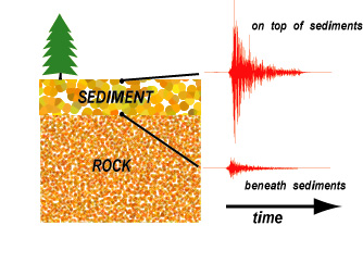 Waves of a small earthquake impinge on the boundary between the rock and overlying sediments (lower seismogram), and become amplified as they travel through the sediments to the surface (upper seismogram). A seismogram records the wave motion over time. (Courtesy of C. Langston, The University of Memphis.) |
Probabilistic ground motion maps represent
the output of a series of computer programs. These programs
simulate the occurrence of earthquakes of various magnitudes, types,
and locations, how earthquakes generate earthquake (seismic) waves and
how these waves travel through the rocks and sediments. We try to
make these simulations as realistic as possible by constraining the
inputs to them with observations from real earthquakes and the
laboratory. The Memphis maps use the same methods and inputs as
the national seismic hazard maps but we add to these a series of
analyses and programs to simulate the effects of the sediments beneath
Memphis. In essence, the national maps calculate motions
expected if the rocks were uniform throughout the Central and Eastern
US
and had no overlying sediments. The Memphis maps add in the
effects
of the sediments (e.g. as in the figure on the left), which vary
significantly throughout the region and even over distances much
smaller
than the city. Here we focus primarily on describing how we include the
effects
of the sediments and only summarize very briefly the entire scheme for
calculating
the hazard maps. We refer you to the extensive
documentation for the national maps for details about all but the
inclusion of the
local geology. |
| At each location on the
map we perform a suite of calculations (recalling the calculations are
done on a grid of points covering the mapped area). In these
calculations we
include the effects
of the sediments by using 'site amplification factors', which
effectively multiply the ground motions expected without any sediments
by an amount calculated for the particular sediment structure found at
the site. As noted above, probabilistic hazard maps account for both what we know and also what we don't know about when and where earthquakes will occur, how they radiate seismic waves, and how those wave travel through the rocks and sediments. Basically at each map location a whole suite of ground motion estimates are calculated using different input parameters sampled from a range of reasonable values. From this suite, the mean estimate becomes the mapped ground motion. When considering the effects of sediments, the first step is to determine what is the range of reasonable site amplification factors. Examples of those derived for Memphis are shown below, followed by a summary of the steps followed to derive them. |
|
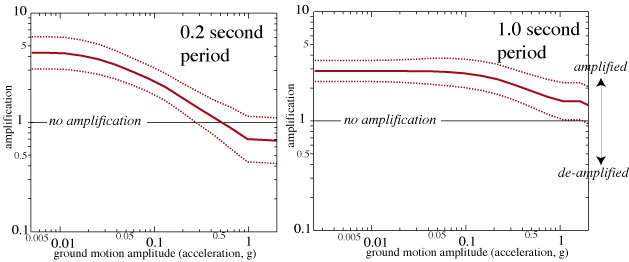 Site amplification ranges
derived for a site in Memphis for ground motions with 0.2 second (left)
and 1.0 second (right) periods. Solid and
dotted red curves
show mean values and the range encompassing 68%
of
all values, respectively. These show how motions with a given amplitude
(measured in acceleration units, along the horizontal axis) may be
amplified or de-amplified by the sediments at this site. For
example, 1.0 second period motions between about 0.002 g and 0.1 g will
be approximately 3 times larger than they would have been if there were
no sediments. Note the logarithmic scales.
|
|
A major part of the effort in generating the Memphis maps went into characterizing the sediment structure. Most important for the ground motion calculations is knowledge of a physical property called 'shear wave velocity', but also a number of other properties. This characterization involved collecting a substantial amount of new information, obtained either by gathering together existing data from a wide variety of sources or actually making our own measurements. Either directly or indirectly this involved numerous participants from the Memphis, Shelby County community and scientists within and outside the USGS. Characterizing the sediment structure begins at the surface, and is accomplished through field mapping of the materials found in exposures throughout the County and displayed in new geologic maps. A simplified version, shown on the right, displays the distribution of wind-blown glacial deposits (called 'loess') and river deposits (alluvium). |
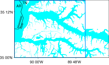 Map of the distribution of the two main types of sediments found at the surface in Shelby County; river (blue) and wind-blown glacial (white) deposits. Current hazard maps cover the area outlined by blue square, but the Collierville quadrangle to the east is shown as the hazard maps may be expanded there. |
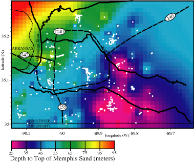 Example of the 3-D variation in sediment structure, showing the depth of the top of the Memphis Sand layer beneath Shelby County, estimated from subsurface logs (white dots). The Memphis Sand is a major aquifer for the city and county. The estimated depths aren't reliable where there are few or no logs. |
While the surficial materials provide some clues about what lies beneath, the thicknesses of the various sediment types varies considerably with depth even if those at the surface are the same. Fortunately others also have had reason to examine what lies beneath, have logged the subsurface using a variety of measurement types, and made the logs publicly available. The two most common types are deeper water well logs and numerous, but shallower, engineering boring logs. We have gathered together as many as of these as possible, interpreted each log in terms of the sedimentary structure at the logged location, and made them all available in a new Shelby County Subsurface database. From these we construct a 3-dimensional representation, or model, of the sedimentary layers. |
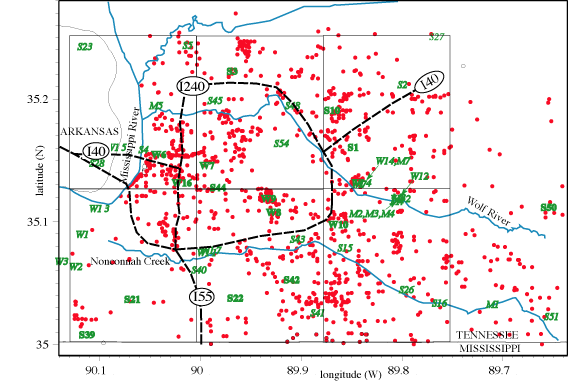 Map showing the locations where logs (circles) and shear wave velocity profiles (letter/number labels) were measured, and major waterways (blue lines) and interstate highways (thick black lines). Rectangles show the six 7.5” quadrangles for which we made hazard maps. |
While the observations are abundant for constraining the sedimentary structure in terms of the sediment types this description isn't exactly what's needed to calculate the expected amplification. Instead, one of the most important things we need to know is a material property called shear wave velocity. This is a measure of how fast certain kinds of seismic waves travel, and its variation mostly with depth determines how much waves will be amplified or de-amplified. Unfortunately such measurements are not simple to make and none existed prior to this project - thus, we measured many tens of new shear wave velocity profiles and have put them in an online database. Not surprisingly, there is a correlation between the sediment types and the shear wave velocities, which we quantify. This correlation allows us to use the 3-dimensional sedimentary structure model determined from the abundant log observations as a basis for interpolating between more sparse shear wave velocity measurements (see left). In this way we can estimate the range of reasonable shear wave velocities anywhere in the mapped region. |
| In addition to depending
on certain material properties, the response of sediments to shaking
depends on the shaking itself. If the waves that shake the ground
oscillate rapidly up and down (i.e. have short periods) the
energy may dissipate more quickly than for slower (longer period) wave
motion, leading to greater de-amplification in the first case.
The sediment response also depends on the strength of the
shaking. If shaken sufficiently strongly, the sediments may begin
to break apart so that waves can no longer efficiently be transmitted
through them. This may have the beneficial effect of limiting the
amplitude of the shaking, but eventually can lead to a catastrophic
phenomenon called ground failure. This complex relationship
between the input shaking and the sediment response is somewhat
predictable and calculable, but still is a source of considerable
uncertainty. To simulate the shaking input to the
sediments we use real earthquake ground motions recorded at sites with
no sediments at all. In this way
we are guaranteed that all the various types of waves and complex
processes that happen to generate and propagate seismic waves are
included. For
our input motions we sample from a suite of 16 recordings.
Because the
amplification factors are calculated for a specific period and
amplitude of
input ground motion, for each calculation we scale the recordings used
so
that they have the desired amplitude at the specified period. |
|
| We illustrate the
effects of the sediments beneath Memphis on the hazard by comparing the
ground motions estimated with and without the sediments. The
latter is what is displayed in the USGS national seismic hazard maps,
which are calculated for what is called 'firm rock' or equivalently at
the boundary of NEHRP (National Earthquake Hazard Reduction Program)
soil classes 'B' and 'C'. This soil classification is often used by
engineers and distinguishes soils partly based on their
average shear wave velocity for the top 30 meters. All of Memphis
falls
within a NEHRP soil class 'D'. We compare below the Memphis and
national
maps showing ground motions with 2% probability of being exceeded in 50
years. |
|
| |
 |
| Probabilistic
hazard maps showing ground motions with a 2% probability
of exceedance in 50 years for PGA (left) and 0.2
second period (right) ground motions. Inset map of Memphis,
Shelby
County includes effects of sediments, superimposed on the larger
national seismic hazard map that does not. Because the strongest ground motions are de-amplified by sediments for rapidly oscillating waves (shorter periods), the ground motions in the Memphis hazard maps are less than those in the national maps for PGA and 0.2 second period motions (above). The thicker sediments in the west result in greater de-amplification of ground motions westward. The ground motions estimated without the effects of the sediments (which can be thought of as the 'input' motions to the Memphis map calculations), shown in the national maps (region outside the Memphis area above), also increase westward because the largest earthquake sources are northwest of Memphis. The net effect of the westward increasing de-amplification also increases westward resulting in ground motions that are more uniform in the Memphis maps than in the national maps. |
|
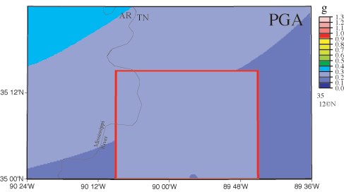
| The tremendous thickness of sediments beneath
Memphis causes amplification for slower oscillations (longer periods).
The thicker sediments in the west tend to amplify the long period
ground motions (as in the 1.0 second period on the right) more in the
west so that relative to the national maps, the Memphis hazard maps
retain a decreasing gradient of ground motion
amplitudes to the southeast. This gradient in the national maps
reflects
the fact that the largest potential earthquake sources are to the
northwest
of Memphis. |
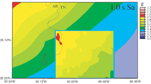 |
| Probabilistic hazard maps
as above, but for 1.0 second period ground
motions. |
|