Seismic Analysis Code 5
This class focuses on using SAC to perform a common signal detection operation: cross correlation. This is another technique to combat poor signal to noise ratios in time series data. The basic idea is to take a known signal and find other times where similar signals occur in a noisy time signal. To perform such signal detection, we will make use of the cross-correlation function in SAC.
Cross-Correlation, Autocorrelation, and Convolution
Common techniques in signal processing frequently make use of cross-correlation, autocorrelation, and convolution operations. These three operations are all related, and involve integrating the product of two functions with a varying time lag. Given two functions \({f(t)}\) and \({g(t)}\), then the cross correlation \({(f\star g)(\tau)}\) of the two functions is defined to be
This can be thought of as a moving inner product between the two signals, where \({\tau}\) indicates the time lag between the two signals. If the cross correlation is large at a given time lag, that means that the two signals are similar when they are offset by that value of the time lag – this is true if the cross correlation is positive or negative, with negative indicating the signs are reversed. If the cross correlation is small at a given time lag, then the signals are different at that given offset.
The autocorrelation is simply the cross-correlation of a signal with itself. The autocorrelation function thus has its maximum at a time lag of zero, and is symmetric about \({\tau=0}\). The convolution \({f*g}\) is also similar, but one of the functions is reversed in time. This is illustrated in the figure below, along with a visual representation of how each function takes the values that it does.
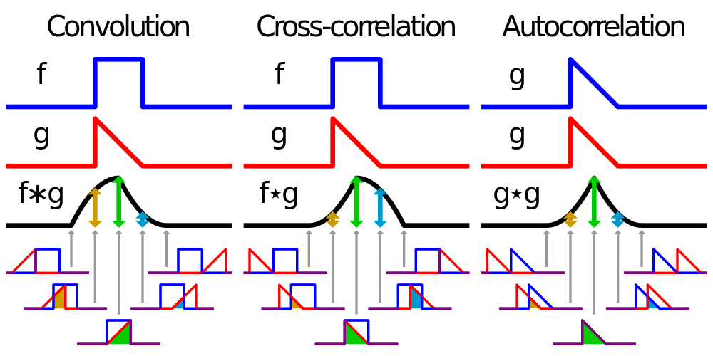
Examples of convolution, cross correlation, and autocorrelation for basic functions. The cross correlation measures the similarity between two signals, while the convolution is essentially a time reversed cross correlation. Autocorrelation measures the similarity of a signal with itself, so it always peaks at zero offset and is symmetric.
Waveform Cross Correlations
SAC can also be used to perform auto- and cross-correlation analysis, which can be combined with stacking as a useful technique for identifying events in a low signal to noise signal. Basically, when the two signals line up in a coherent way, the cross correlation is larger. This can be used to isolate signals from noise, particularly if multiple stations and components are stacked to find situations where several different signals find something similar. Correlations can be easily computed in the frequency domain using Fast Fourier transforms – while a cross correlation in the time domain requires \({N^2}\) operations (where \({N}\) is the length of the signals), in the frequency domain this only requires \({N}\) operations. However, we have to do the FFT in order to accomplish this, which requires \({N\log N}\) calculations, so the overall dependence on the signal length is \({N\log N}\). Regardless, this is an improvement over the time domain calculation, so using this trick cross-correlations can be computed quickly even for long signals.
To calculate a cross correlation in SAC, we use CORRELATE. Correlate requires that at least two signals be loaded into memory. We need to choose which of the signals to treat as the “master” and this is designated by the order in memory. If we want the first signal to be the master then we enter correlate master 1, while if we want the second signal to be the master we type correlate master 2. SAC will then correlate the master signal with all signals in memory. Thus if the master is 1, then the first signal in memory will be the autocorrelation of the first signal, while the second signal in memory will be the cross correlation between the signals.
Exercise: Calculate the cross correlation of a boxcar and a triangle function. While the triangle function is not quite the same as in the previous figure, you should see similar results. Also calculate the autocorrelation of each function to verify that the peak is at a time lag of zero and it is symmetric in time regardless of the input function.
Cross correlation can be used to take a known signal and find times when that signal reoccurs in another set of data. It frequently works even if there is a large amount of noise, particularly if many waveforms are used and the results are stacked. The idea is to cross correlate the known signal with a long time series and find times when the cross correlation is large (meaning that the two signals are similar, and thus detect a similar occurrence to the previous event). While the cross correlation may not be high for one particular signal, if we stack many signals we can further improve the signal to noise ratio.
Exercise: I have included a series of 6 waveforms for you to try implementing this method (they are all in the zipped tarball waveformcc.tar.gz). The first three are a set of waveforms for a small earthquake in Northern California (template1.sac, template2.sac, and templateZ.sac for the two horizontal and vertical components). These are waveforms recorded on a nearby seismometer. I have also included a recording of another small event that occurred close by where I added noise that completely drowns out the signal (noisy1.sac, noisy2.sac and noisyZ.sac). Your goal is to write a macro that uses the template waveforms to detect the earthquake in the noisy data.
Hint: Cross correlate each component of the template waveform with the corresponding component of the noisy signal. Write the resulting cross correlations to disk, and then stack them. It is helpful to remove the mean of the data before doing the correlation by using rmean as it makes the cross correlation values more stable. Once the cross correlation function for all three components are stacked, you should be able to clearly see the time at which the event occurred on the resulting signal (the stacked cross correlation should show a large spike at the time of the event, see below). Plot the data as needed to see what is going on.
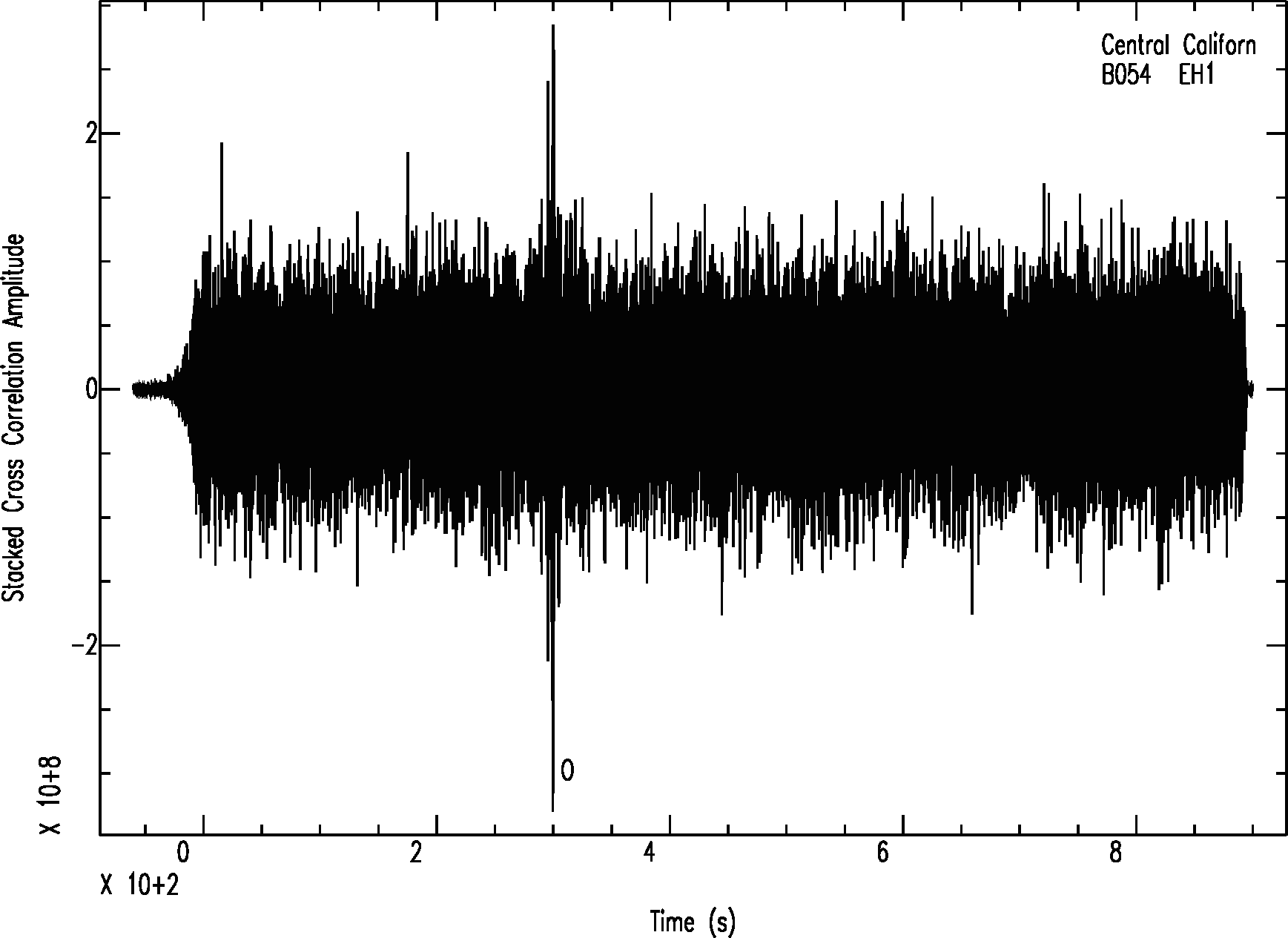
Note that this is only for three components; repeating this operation over many stations will further improve the signal to noise and make the event detection even more clear. This is a frequently used method to improve detection of seismic events: using previously detected catalog waveforms, this method can quickly scan long time signals and detect the time of any additional events with similar waveforms.
This lab illustrates how we can use simple features in SAC to perform more complicated signal processing tasks. While we have not covered all aspects of SAC, hopefully you should have a working knowledge of how to use it and can figure out how new commands work from the manual. There will be one homework assignment using SAC, which will involve downloading waveforms, rotating components, decimating/filtering, and plotting what is known as a record section.