Seismic Analysis Code 2
This lab focuses on additional material relating to graphics in SAC, and how to write SAC macros (which are essentially scripts to carry out a series of SAC operations, allowing you to conduct more complex computations using SAC).
Details about SAC Plots
Quick and Dirty Plots
Run SAC on your computer, and load one of the seismograms that you downloaded for the previous class, and plot the function. Your plot should look something like this:
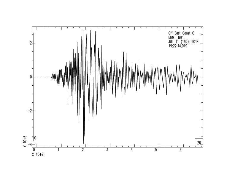
Notice the box in the lower right hand corner– for my plot, it says “26” but depending on the length of the signal that you plotted you will see a different number. This number signifies that SAC is only plotting every 26th point in this graph.
Why does SAC do this? On the original Tektronix system, the data transfer rate is painfully slow, to the point that displaying a plot of seismic data at a typical sampling frequency would take several hours. Thus, by default SAC desamples long time signals before plotting them in order to reduce the time needed to transfer the data to the display.
Unfortunately, this is not implemented very well. When SAC performs this operation, it simply desamples the data, taking very few points. This is unlikely to give accurate information about the amplitude of the signal (because the probability that the maximum value of a particular wiggle is displayed is only 1/26), and means that the plots are not particularly useful for analysis (particularly for very long signals with many data points, which would require even more aggressive desampling). A better way to do this would be to take the maximum value within every desampling window and plot that value, making the signal amplitudes useful (referred to as decimation). While it requires an additional processing step, the time required to do this extra processing step is minimal compared to the data transfer time on the original Tektronix display.
Fortunately for us, since we have modern computers with modern displays, we do not have to worry about long times to display signals. To prevent this behavior in SAC, we need to turn off the “quick and dirty plot” option (which is set to “on” by default. If you type qdp off into the command line and then plot your data again, you will see a plot with no number in the corner:
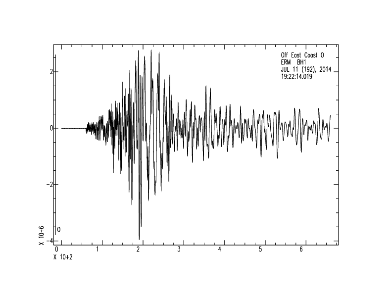
This plot has information that accurately reflects the signal amplitude (and notice that the display time was not noticeably different than before), though for us the amplitudes aren’t markedly different. If you are going to use SAC plots for any real scientific purpose, turn off the quick and dirty plots!
Labeling Axes and Titles
To label axes in SAC, use the XLABEL or YLABEL command. The syntax is xlabel on '<label>' for the \({x}\)-axis (similar for the \({y}\)-axis. For example, if I wanted my \({x}\)-axis to be labeled as ‘Time (s)’ I would type xlabel on 'Time (s)' into the terminal. As you may remember, this will have no effect on the current plot until you issue the plot command again, so you need to issue these commands before plotting for them to take effect.
To add a title, use the TITLE command. It is issued in the same way as the xlabel command, so to title a plot, type title on 'Seismogram' to add the title ‘Seismogram’ to your plot. Again, you will not see any effect from the title command until you issue the plot command.
Changing the Plot Appearance
We have already discussed how to change the limits on a plot and how to make a color plot, but there are additional customizations that are possible. To change the spatial size of a plot, use the XVPORT and YVPORT commands. The syntax is xvport <min> <max>, where <min> and <max> are numbers between zero and one that specify the minimum and maximum values of the axes as a fraction of the entire plot window. The default values of xvport are 0.1 and 0.9, and the default values of yvport are 0.15 and 0.9. To make a smaller plot, I would issue the commands xvport 0.1 0.5 and yvport 0.15 0.55 and then the plot command.
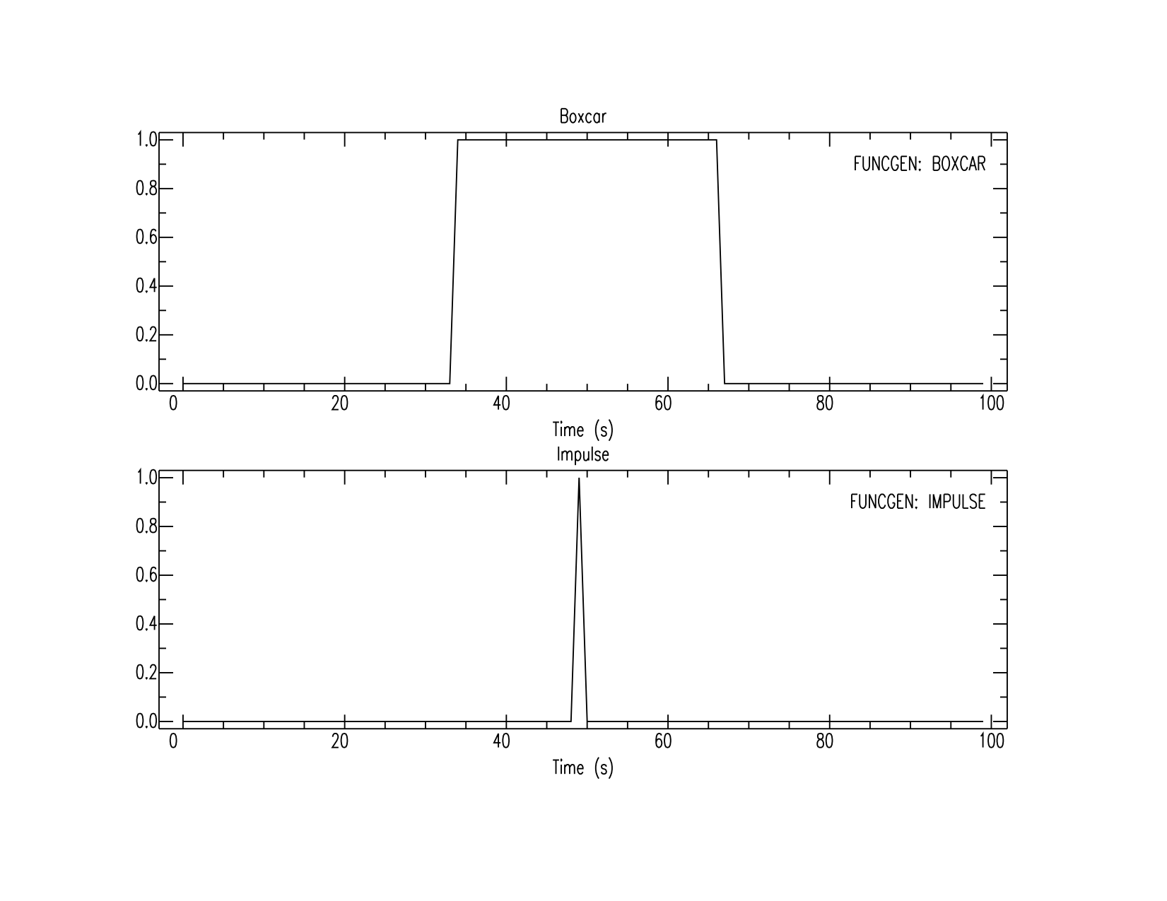
To put multiple plots in the same figure, we use the xvport and yvport commands in conjunction with the BEGINFRAME command (shortened to begfr). When you enter the beginframe command, SAC will add a new axes to the existing figure when subsequent plot commands are issued, rather than making a new figure. Thus, once we enter the beginframe command, we can add plots in specific locations by setting xvport and yvport and then giving the plot commands. When the ENDFRAME command is issued, the default behavior resumes. An example to make a plot with two axes is:
beginframe
xvport 0.1 0.9
yvport 0.15 0.475
funcgen impulse
title on 'Impulse'
xlabel on 'Time (s)'
plot
xvport 0.1 0.9
yvport 0.575 0.9
funcgen boxcar
title on 'Boxcar'
xlabel on 'Time (s)'
plot
endframe
Saving Plots
So far, we have been making plots and displaying them on the screen. What if we want to save a plot for use in another document?
The simplest way to save figures from SAC is to use SAVEIMG to directly output a figure window to a standard graphics format. This command is flexible and will let you save the currently displayed figure window to PDF, PS, or PNG formats without doing any additional work. Once you have a figure up and displayed, simply enter saveimg <filename>.<format>, where <filename> is your desired name for the file and <format> denotes the extension of the graphics format that you wish to use. Thus for example, to plot an impulse function and save as PDF, you would do the following:
funcgen impulse
title on 'Impulse'
xlabel on 'Time (s)'
plot
saveimg impulse.pdf
This has the advantage over the more complicated procedure described below in that the labels are rendered as text rather than as lines. Because of this, I would generally advocate using saveimg to produce plots.
However, if you are interested in more details about producing graphics in SAC, there is another procedure that gives you a bit more control. SAC has its own graphics format, known as ”.sgf” (SAC graphics format). This format is analogous to the MATLAB ”.fig” files as they only readable by SAC, and is not useful if we want to include the figure in other documents like presentations, posters, or papers. To save a plot in the ”.sgf” format, we need to follow a few steps.
SAC has two different output devices. A device is just a fancy name for the destination where the graphics will be displayed. So far we have used the screen as our output device, but we have the ability to tell SAC to send our plots to a different device. To use the screen as an output, we use the XWINDOWS device (can be abbreviated x). You may have noticed so far that when we issue a plot command, the plot window shows up in an application called “X11” which is the xwindows application for a Mac.
The other available output device is SGF, or SAC Graphics Format. If we choose this output device, plots will not be displayed on the screen, but instead will be written to file. To change the output device, we use the BEGINDEVICES command (bd in shorthand). By default, the device is set to xwindows, but by typing begindevices sgf, all future plots will be saved to file as an ”.sgf” file instead of being displayed on the screen. To switch the device back to the screen, type begindevices xwindows.
When you use the sgf device, each plot command that you execute will save to a new sgf file. The first plot after you start SAC will be saved to “f001.sgf” in your current working directory. Subsequent commands will save as a file with the name “f002.sgf,” “f003.sgf,” etc. If any file already exists (say from a previous SAC session), then it will be overwritten without a warning, so if you want to save your sgf files, you will need to rename them after each SAC session.
To convert an sgf file into a graphics format that is useful outside of SAC, we use the sgftops utility (note that I called sgftops a utility, as it is not an official command in the same sense that plot and read are commands). This converts an sgf file to PostScript, which is a standard graphics format that can be opened with Applications such as Preview on the Mac (when Preview opens a PostScript file, it automatically converts it to PDF), Adobe Illustrator, or on the command line using ghostscript. To convert a file, use the syntax sgftops f001.sgf sacplot.ps which converts the sgf file “f001.sgf” to the file “sacplot.ps” which can then be viewed in another application.
There are two additional options when using sgftops that you can include in the command. The first specifies the line thickness in the resulting PostScript file (the default value is 1), and the second allows you to specify the page layout or add an id that specifies some details about the plot. To add an id, make the second option i, to change the page layout specify s, or si for both. The s option is useful if you want your plot in portrait rather than the default landscape mode – this option will prompt you to enter specific values for the \({x}\) and \({y}\) translations (relative to the lower left corner of the page, assumed to be US Letter size in portrait orientation), rotation (measured counterclockwise from horizontal), and scale. An example, to obtain a plot with thicker lines type sgftops f001.sgf sacplot.ps 1.5 into the command line. To rotate and scale the plot into portrait mode, use sgftops f001.sgf sacplot.ps 1 s and then at the prompt, type the following four numbers, each followed by a carriage return: 0.5 0.5 0 0.75. This will result in a plot in portrait mode.
As you can see, this requires considerably more effort than using saveimg without a huge difference in the final outcome. Because of this, I do not use the SGF procedure much any more, and simply use saveimg to save figures in SAC.
Exercises: Try out some of the plot commands described above. First, plot a seismogram with the quick and dirty plot option off. Then, plot a seimsogram with labeled axes and a title, save it as a PDF file. Compare with the results using an SGF file converted to PostScript. Finally, use beginframe along with xvport and yvport to illustrate four of the different functions created by funcgen in a 2x2 grid of plots.
SAC Macros
Like with MATLAB .m files, we can write scripts to carry out a series of commands, called “macros” in SAC. SAC macros are text files containing a series of commands that can be called either from within SAC or directly from the command Terminal.
For example, here is a series of commands. Enter them into a text file (using an editor of your choice), and then launch SAC. You can name the file whatever you like, but I prefer to include .macro at the end so that I know that the file is a SAC macro. From inside SAC, type macro test.macro (using the name that you chose for your file) to execute the macro. For example,
# SAC macro to generate three functions, write to disk, and plot
funcgen impulse
write impulse.sac
funcgen boxcar
write boxcar.sac
funcgen triangle
write triangle.sac
read impulse.sac boxcar.sac triangle.sac
plot1
# and * serve as comment characters in SAC, so that line will not be executed. However, you cannot put inline comments into SAC, so comments must be on their own line. Alternatively, you can run the macro from the Terminal by typing sac test.macro directly from the command line.
Input Arguments
While this type of macro is easier than typing a series of commands into the command line (where you are likely to make a mistake if you are not careful), macros are more useful when they can take input arguments like a function in MATLAB or Python. SAC macros do not have an explicit way to write functions, but you can pass an arbitrary number of arguments to any SAC macro, and the parameters will be available using the variables $1, $2, etc. As a simple example, if we wanted to write a macro to read three SAC files and plot them, change your macro to the following:
# SAC macro to read three files from disk and plot
read $1 $2 $3
plot1
If you type macro test.macro impulse.sac boxcar.sac triangle.sac into the command line. You should get the same plot as before. If you call the macro without specifying any arguments, you will get a prompt asking you to input the arguments.
What if you want to read an arbitrary number of SAC files? You can make the macro more flexible by specifying keywords, which can take an arbitrary number of arguments. Change your macro to the following:
# SAC macro to read an aribtary number of files from disk and plot
# files to read are set using the "files" keyword
$keys files
read $files
plot1
By typing macro test.macro files impulse.sac boxcar.sac into the command line, you can run this macro, and you can change the number of input files to whatever you like without changing the macro. If you do not give any values for files, SAC will prompt you to enter the values (Note: I have found that this does not always work on SAC installed in the Mac Lab, so you may end up getting an error if you do not provide the input arguments).
You can also specify default parameters. If you want your macro to plot impulse.sac, boxcar.sac, and triangle.sac by default, then change the macro to:
# SAC macro to read files from disk and plot
# files to be read are set using the "files" keyword
# if no files provided, default files are impulse.sac boxcar.sac triangle.sac
$keys files
$default files impulse.sac boxcar.sac triangle.sac
read $files
plot1
Now you can run your macro with any number of arguments, or with no arguments to plot those three functions by default. (Note that I have also found that setting default parameter values does not always work correctly in the Mac Lab for some reason, so you may sometimes get an error when doing this in the Mac Lab.)
Variables
One of the valuable aspects of any programming language is the ability to assign values to variables. This can be done in SAC using what is known as a “blackboard” variable. You can set a blackboard variable using the SETBB command, followed by the variable name and the value. For example, setbb xmin 40 will define a variable xmin with the value 40. To access the variable, use %xmin.
You can also calculate other parameters from variables, which you can do using the EVALUATE command. Let’s say that we want a macro that will plot an arbitrary number of functions from an arbitrary starting time for 100 seconds. We will have keywords for the entries for xmin and files, or
# SAC macro to read files from disk and plot with a time range of 100 s
# files to be read are set using the "files" keyword
# if no files provided, default files are impulse.sac boxcar.sac triangle.sac
# also must provide argument xmin to set start time on plot
$keys xmin files
$default xmin 0
$default files impulse.sac boxcar.sac triangle.sac
setbb range 100
evaluate to xmax $xmin+%range
read $files
xlim $xmin %xmax
plot1
Run this by typing macro testmacro.txt xmin 25 files impulse.sac boxcar.sac triangle.sac to plot the three functions from 25 to 125. The first line defines that input arguments for xmin and files should be provided, then it determines xmax by adding 100 to xmin. Then, the macro reads data from the files, sets the \({x}\) limits, and plots the signals.
Sometimes, you might want to use an input argument or a blackboard variable to represent a part of a file name. A common example might be if you are reading data froma a seismic network, and the file names are identical with the exception of one piece representing the station name or the component in question. To use a variable within another string, you need to append the variable name with the same character that is used to access its value. So for example, let’s say you have two stations, S1 and S2, with components N, E, and Z, and the filename convention from the network operator is stationS1N.sac, stationS1E.sac, stationS2Z.sac, etc. The following macro would correctly read the file specified by the stat and comp inputs:
# SAC macro to read a station component from disk and plot
# must input the station name and component when calling
$keys stat comp
read station$stat$$comp$.sac
plot
This can be called using macro test.macro stat S1 comp N. Similarly, if comp was stored as a blackboard variable instead of a keyword, the equivalent read command would be read station$stat$%comp%.sac. This is very handy when complicated, but predictable, filenames are used that only differ in a couple of arguments.
If statements
Macros can use if statements, with a syntax very similar to that of MATLAB. Let’s say that in the above macro, you only want to change the \({x}\) limits if xmin is greater than zero. In that case, we could use an if statement:
# SAC macro to read files from disk and plot with a time range of 100 s
# files to be read are set using the "files" keyword
# if no files provided, default files are impulse.sac boxcar.sac triangle.sac
# can also provide argument xmin to set start time on plot (default 0), only works if positive
$keys xmin files
$default xmin 0
$default files impulse.sac boxcar.sac triangle.sac
setbb range 100
if $xmin gt 0
    evaluate to xmax $xmin+%range
    xlim $xmin %xmax
else
    xlim 0 %range
endif
read $files
plot1
This will set the limits differently if xmin is negative (gt stands for greater than). Other comparisons available inlcude lt (less than), le (less than or equal to), ge (greater than or equal to), ne (not equal), and eq (equal). The else (or elseif) is optional.
Loops
There are several ways to execute a loop in SAC. The first option is to loop over numeric values (like in MATLAB or using range in Python). Let’s say you have a series of 10 .sac files, with names “signalx.sac”, where x is a number from 0-9. To read all 10 files in using a loop, we can do so as follows:
# SAC Macro to read in 10 files and plot
do i = 0, 9
    read more signal$i$.sac
enddo
plot1
This will read in all 10 files and plot them all on the same axes. Optionally, you can add an increment using do i = 2, 8, 2 to increment by 2 each time. Another way to write this is to use the syntax do i from 2 to 8 by 2.
If you want to loop over a specific set of items, the syntax is a bit different. If we wanted to read all three components of a particular station and plot them, we might modify the above example to be the following:
# SAC macro to read 3 components of a station from disk and plot
# must input the station name when calling
$keys stat
do comp list N E Z
    read more station$stat$$comp$.sac
enddo
plot1
This version explicitly loops over all three components specified by whatever follows list.
If you want to get some files from the shell using a particular pattern, you can loop over files matching a certain pattern, which is very useful for reading in files. In particular, if you wanted to load the vertical component of any station in the current directory, you can do
# SAC macro to plot vertical components in the current directory
do file wild station*Z.sac
    read more $file
enddo
plot1
You can also specify a directory other than the current one if you use do <variable> wild dir <directory> expr.
Finally, you can do a standard while loop in SAC. The syntax is while <condition> ... enddo, and break will work as we have seen previously in Python and MATLAB to exit loops.
Summary
While programming in SAC is a bit less refined than programming in Python or MATLAB, it still lets you get the job done fairly well if your work requires processing .sac data files.
Exercise: Write a SAC macro that generates three sine functions with the same frequency and a fixed phase difference between them. Plot all three functions on the same axes, using a different color for each function. The frequency and the phase offset should be specified through command line variables, as should the number of points and the time spacing used in generating the signal. Default values should be 100 time points, time spacing of 0.05 s, and a frequency of 1 Hz (there should not be a default for the phase offset).