Generic Mapping Tools 1

This is the first of several labs on the Generic Mapping Tools (GMT). GMT is a set of Unix commands for drawing maps and plotting geophysical data on maps, though you can also use it to make basic x-y plots. GMT is a common tool used by many geophysicists.

About GMT

GMT is a collection of open-source tools for manipulating geographic data and producing plots and maps. The GMT tools were originally created by Paul Wessel and Walter Smith, though now there are several more developers involved in maintaining and adding new features. GMT features 25 different map projections, and tools to plot a variety of different types of data on them. GMT follows the Unix philosophy (small programs that do one thing well; string together several programs to do complex things), which makes it very powerful (you have control over every detail of your plot) and difficult to learn (you have to specify every detail of your plot).

Additional mapping tools are available in addition to GMT. MATLAB has a mapping toolbox (I have never used it, so have no idea how useful it is). I have used the Python Basemap and Cartopy packages in my research and found that they produce results on par with GMT. Because of its large usage, high quality output, and free and open source availability, GMT is a very useful tool in geophysics research, which is why we cover it in this class.

GMT commands are typically combined in a shell script. While they can be used interactively from the command line, they are quite complex to type out, making a shell script a convenient way to use them. Additionally, because many maps are built up in a similar way, this means you can often reuse scripts with some simple modifications for the particular map that you would like to make. This is particularly the case if you use shell variables to form commands. Using shell variables in your commands provides a number of advantages. First, GMT commands are often difficult to understand, but using shell variables means that you can use descriptive variable names to remind you of what everything is doing in a GMT command. Additionally, re-use is easier, as you can set apart the variable definition and command execution so that you can focus on setting parameters and not have to change the parameters, increasing the chances that you get correct code.

I have found that the best way to learn GMT is to get a hold of some example scripts and modify them to figure out what is going on (incidentally, this is how I learn how to use pretty much any type of computing tool). For each lab on GMT, I will provide a shell script that makes a few different maps. You should run them yourself to confirm that they work, and then change some of the shell variables to understand how they work. GMT has extensive documentation (I find myself reading the manual online on a frequent basis), though those pages are often incomprehensible when there are many options to specify.

GMT is currently on version 5. This is the version installed in the Mac Lab, though some older machines may still have GMT 4 as the latest version. Further complicating things is the fact that the Mac Lab lets you use the GMT 4 method for denoting command names, even though it is calling GMT 5. Having these two different versions makes things tricky because the GMT developers decided to change the syntax for a number of commands in going from GMT 4 to GMT 5. The shell scripts I provide can be used for GMT 4 or 5 (I do this by using shell variables and setting them to appropriate values depending on whether GMT 5 is detected on the system), but it is not necessary for you to do this in your homework – I just provide these to illustrate how you might make your scripts work for multiple versions. I will introduce the differences between GMT 4 and 5 as we proceed.

A Basic Axis Frame

The provided shell script gmt1.csh will produce three plots: gmt1_1.pdf, gmt1_2.pdf, and gmt1_3.pdf. Each one contains a number of comments explaining the GMT commands and options. Read through the comments for the first set of commands in the script, which produces the plot gmt1_1.pdf, shown below.

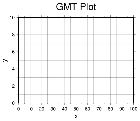
This is just a basic axis frame – since GMT follows the Unix philosophy, making axis frames and plotting data are two separate operations, and thus require separate programs. Here is the GMT 4 command that made this plot:

psbasemap -R0/100/0/10 -JX4i/3i \
    -Ba10f5g5:"x":/a2f1g1:"y"::."GMT Plot":WSne -P > gmt1_1.ps

And in GMT 5, the command is

gmt psbasemap -R0/100/0/10 -JX4i/3i \
    -Bxa10f5g5+l"x" -Bya2f1g1+l"y" -BWSne+t"GMT Plot" -P > gmt1_1.ps

Note that these are pretty incomprehensible by themselves. To make this easier to read, I define a number of different shell variables containing the relevant information and give them descriptive names. With the shell variables, this is actually

set code = "psbasemap -R${xmin}/${xmax}/${ymin}/${ymax} -JX${size} ${bvals} $portrait > $outfile"
eval "$code"

Note how this is easier to understand, and it allows you to define all the pieces you need without looking at the command to figure out where everything goes.

One thing to note: when executing these GMT commands, I define shell variables to be strings containing double quotes for any axis label so that when they are substituted into other commands, the quotes remain behind so that GMT can figure out what my axis labels are. However, you do not need to include the quotes if your labels do not contain spaces – they are only strictly necessary if you want to have spaces in your labels or title.

However, if you just try to put shell variables containing spaces inside of quotes into shell command using variables, the shell trips up on them, mistaking the space for the start of a new flag. To avoid this, I put the entire command into a separate shell variable, and then use the eval command to evaluate the entire quoted shell variable. This ensures that the shell literally interprets exactly what I want as an entire string forming a single command. This is not needed if there is no label containing spaces, so if you are wondering why some of my plots use this method while others do not, this is why.

The details of how to draw this plot are specified by all of the various command line options above. We will go through these one at a time to explain them.

1. First is the psbasemap command. In GMT 4, you simply call psbasemap, while in GMT 5 you need to put gmt before the command name. I am able to use psbasemap in either case by defining an alias at the beginning of the script if GMT 4 is not detected on the system. In the Mac Lab, we use GMT 5 but these aliases are already defined, so you can use either version in your own scripts. This is the command to produce an axis frame, though it does not plot any data (that is a separate commamnd).

2. -R0/100/0/10 R here stands for “region” and tells GMT the range of the plot. Note that unlike MATLAB, GMT does not assume anything about our plot, including the fact that we want our plot to show all of the data. We have to set it ourselves for every plot. Here, this says that we want the \({x}\) range to go from 0 to 100, and the \({y}\) range to go from 0 to 10. R is one of the required options for the psbasemap command. Note that when I use it, I set up shell variables for the min and max for each axis so that I can set the limits in a way that is easier to understand.

3. -JX4i/3i J specifies the projection (I do not have a mnemonic to remember the meaning of J). In this case, X means that we are plotting an \({x}\)-\({y}\) plot, and that we will tell GMT the plot size (you can alternatively give a lower case x which signifies that you want to specify the scale per unit). Here we give 4i, which means the \({x}\)-axis should be 4 inches long, and 3i means the \({y}\)-axis should be 3 inches long. J is also a required argument for psbasemap. Note that I use a shell variable for this as well, so that I know what to change if I want to alter the size of my plot later.

4. -B The B option (“boundaries”) is probably the most complex and confusing of all of the GMT options. It tells GMT how to label the axes, how to draw grid lines, and how to title the plot. The manual for B is nearly incomprehensible as far as I am concerned, but hopefully you can figure out by trial and error by modifying the example here to see how it works.

   This is one of the other places where GMT 4 and 5 differ. I account for this by putting all of the B options in a shell variable that is set depending on the version that is detected.

   There are several parts to the -B command in this example:

   • a10f5g5:"x": the first part of the option prior to the slash specifies how to draw and label the \({x}\) axis. You can then give any of three letters a, f, and g, each followed by a number, which describes the annotations (a), ticks (f), and grid lines (g). The number following each of them determines how frequently each item is drawn. Finally, :"x": says to label the axis as “x”. There are more options beyond these, which you can try to decipher from the manual.
   • a2f1g1:"y": does the same thing for the \({y}\) axis as was done above for the \({x}\) axis. If you want both axes to be annotated in the same way, then you do not need to provide the forward slash and the second set of annotation commands. However, if you want different labels for each axis, you need to give both options, even if the annotations are the same.
   • :."GMT Plot": This additional text gives the title. Note that the period prior to the text signifies that this is the title and not an axis label.
   • WSne These trailing letters determine how GMT will draw the axis frame. The letters W, S, n, and e each stand for the west, south, north, and east borders, respectively. If a letter is capitalized, that means to both draw and annotate the border. If it is lower case, then that means to only draw the border. If that letter is not present, then GMT neither draws nor annotates that border. Note that you must draw at least one border, so if you call B with no letters, it will draw and annotate all four by default.
   • For GMT 5, you must call -B a separate time for each axis to be annotated, plus once more to set the display of the axis frame and title. If the first letter of the -B call is x, then that is for the \({x}\)-axis, if y is the first letter then you are annotating the \({y}\)-axis, and if there is no x or y then that call will set the frame. Labels and titles are preceeded by +l or +t, respectively and must appear in the -B call starting with x or y for a label, and without for the title. Hopefully the included examples make this more clear.

   As you can see, B is very complex and can be difficult to understand. This is why I generally set everything in B through shell variables so that I have a much clearer picture as to what is going on. You should try experimenting with the options on this script until you get an idea of how they work.

5. The final option is -P, which says to make the plot in portrait mode (default is landscape, which will be rotated by 90 degrees from vertical). I generally use portrait mode for all my maps, so there is a -P in all of my commands. However, to make it easier to toggle portrait mode on/off, I define a shell variable portrait that is included with every call. To enable portrait mode, I include set portrait = "-P" in the shell script, and set portrait = "" to turn it off. This way, it is set in one place and you do not have to go looking for -P flags to delete from every command.

6. The file is then output to gmt1_1.ps, a postscript file. Because most GMT commands write output to a file more than once, it is a good idea to use a variable for this so that you only have to set it once. PostScript is the default output format of GMT. You can use Preview on the Mac to open PostScript files and convert to PDF and other formats. GMT also provides a command ps2raster (GMT 4 and some versions of GMT 5) or psconvert (later versions of GMT 5) to convert PostScript to other formats, which I use here. There are many options for psconvert: here I use -A0.1i which says to crop the image 0.1 inch around the edge, and -Tf says to give PDF output. See the manual for other output format options with psconvert. I also delete the postscript file when I am done with it, as the PDF is easier to deal with for viewing.

You should tweak the commands within this script to see how it changes the final plot appearance. Try changing one thing at a time, in all three of R, J, and B (using the shell variables that I defined). When you have an idea of how this works, proceed to the next plot to see how to actually plot some data.

A Basic Plot

The second portion of the shell script produces a plot that shows some actual data, and outputs the file gmt1_2.pdf. This plot requires three separate commands to produce the following output:

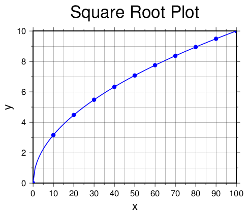
Here is the full set of commands for GMT 4:

psbasemap -R0/100/0/10 -Jx0.04i/0.3i \
    -Ba10f5g5:"x":/a2f1g1:"y"::."Square Root Plot":WSne \
    -X2i -Y3i -K -P > gmt1_2.ps
awk "BEGIN { for (x = 0; x<=100; x++) { print x, sqrt(x) } }" | \
    psxy -R -J -W1p,blue -K -O -P >> gmt1_2.ps
awk "BEGIN { for (x = 0; x<=100; x += 10) { print x, sqrt(x) } }" | \
    psxy -R -J -Sc6p -Gblue -O -P >> gmt1_2.ps

For GMT 5, the commands are:

gmt psbasemap -R0/100/0/10 -Jx0.04i/0.3i \
    -Bxa10f5g5+l"x" -Bya2f1g1+l"y" -BWSne+t"Square Root Plot" \
    -X2i -Y3i -K -P > gmt1_2.ps
awk "BEGIN { for (x = 0; x<=100; x++) { print x, sqrt(x) } }" | \
    gmt psxy -R -J -W1p,blue -K -O -P >> gmt1_2.ps
awk "BEGIN { for (x = 0; x<=100; x += 10) { print x, sqrt(x) } }" | \
    gmt psxy -R -J -Sc6p -Gblue -O -P >> gmt1_2.ps

Using the variable names instead, here is the actual code in the shell script

set code = "psbasemap -R${xmin}/${xmax}/${ymin}/${ymax} -Jx${scale} $bvals -X$xshift -Y$yshift $firstplot $portrait > $outfile"
eval "$code"
awk "BEGIN { for (x = ${xmin}; x<=${xmax}; x++) { print x, sqrt(x) } }" | \
    psxy -R -J -W${pen},$color $midplot $portrait >> $outfile
awk "BEGIN { for (x = ${xmin}; x<=${xmax}; x += 10) { print x, sqrt(x) } }" | \
    psxy -R -J -S${symb}${symsize} -G$color $finalplot $portrait >> $outfile

psbasemap contains some of the familiar options from above, plus a few extras. In this case, R is the same as before, as is B. The J option is slightly different than before, as I have used a lower case x to tell GMT that I am making an \({x}\)-\({y}\) plot. When you use a lower case letter for the map projection, you will specify a scale rather than an absolute size. Here I would like the plot to be the same size as before. Since \({x}\) goes from 0 to 100, then if each \({x}\)-unit is 1/25 of an inch (or 0.04i) the total plot will be 4 inches wide. Similarly, \({y}\) goes from 0 to 10, so to make a 3 inch high plot, each \({y}\)-unit should be 3/10 inch.

I have also moved the plot from the lower left corner of the page using -X2i -Y3i, which tells GMT to place the plot 2 inches to the right and three inches above the lower left corner. Once you call -X and/or -Y, you do not need to call them again in subsequent plotting commands.

Finally, I intend to combine several plotting commands to make a complex plot. To do this, we add the -K option on psbasemap (I think of this as standing for “Keep open”). This allows you to call additional commands to add more things to the plot. I like to handle this using shell variables – I include set firstplot = "-K" and then put $firstplot into the first command in the sequence so that I have a descriptive reminder as to what that option is doing.

Next, we plot the actual data on the plot using the psxy command, which is for plotting \({x}\)-\({y}``\) data. psxy can either read data from a text file, a binary file, or standard input. Here I provide the data using standard input using AWK. First, I use AWK to print out 100 \({(x,y)}\) pairs consisting of \({x}\) and \({\sqrt{x}}\), and pipe that into psxy.

psxy has many of the same options as psbasemap, and fortunately we do not need to specify them every time. If we just give -R -J, then GMT knows to use the same settings as we used in psbasemap. We give four additional options on psxy: -W -K -O -P, two of which we have seen before. -O (I think of it as meaning the file is already “Open”) tells GMT that we are appending plot items onto an existing plot. As with the first plot, I define a shell variable for all the intermediate plots $midplot that handles the -K -O for me. -W gives information on how to draw the lines in the plot: -W1p,blue says that the lines should be 1 point (1/72 inch) wide and blue. All of this is appended onto the existing file “gmt1_2.ps” using Unix output redirection. Also note that in my AWK program, I used double quotes so that the \({x}\) limits are correctly substituted into the program before execution.

Finally, I want to also plot symbols on the figure in addition to the lines. This requires calling psxy a second time, as in the GMT Unix philosophy, plotting lines and plotting symbols are two separate operations. I only want to put a marker for every 10th data point, so I modify my AWK program to only print out every 10th point. You can also change the sampling rate of a dataset using the sample1d GMT command if you were making a plot from a text file – see the manual for more details.

I pipe my AWK results into psxy again. This time, I call two new options for psxy: -S and -G. -Sc6p says to plot each data point as a symbol that is a circle with a diameter of 6 points (6/72 in). -Gblue says to color the symbols blue. Note that we did not call the -W option here – since we gave the -S option, -W refers to the outline of the symbol, rather than lines connecting the points. The symbol outlines are drawn by default, so if you do not want the symbol outlines drawn you need to call -W0 to make the line width zero. Here we want them drawn in the same color as the markers, so we do not need to do anything for -W. As with the previous command, we also call -R -J with no additional text needed, and -O -P to make a portrait layout and tell GMT that we are appending to a previous plot. In the shell script, the -O option is handled by a variable $finalplot so that it is easier to understand what is going on. Finally, we append to gmt1_2.ps as before. I convert to PDF and delete the postscript file when I am done with it.

As you can see, because we need to specify every single detail about our plot, even a basic plot requires a number of commands that can be difficult to understand if you are not GMT savvy. I try to make things easier to understand using shell variables for as many details as I can manage. Anything that is used more than once should always be defined in a shell variable so that it only has to be changed in one place, and anything that is hard to understand is usually better being replaced with a descriptive name that is set separately. Look through my use of variables to see how they can make GMT scripts easier to understand.

Nonlinear Axes

The final example shows how to make nonlinear axes and put text annotations on a GMT plot. The final plot produced by the shell script is the following:

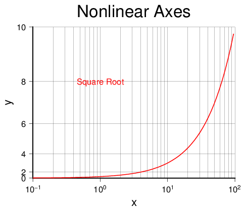
The GMT 4 commands to make this plot are as follows:

psbasemap -R0.1/100/0/10 -JX4il/3ip2 \
    -Ba1g3p:"x":/a2g1:"y"::."Nonlinear Axes":WS -K -P > gmt1_3.ps
awk "BEGIN { for (x=0.1; x<=100; x = x*1.1) { print x, sqrt(x) } }" | \
    psxy -R -J -W1p,red -K -O -P >> gmt1_3.ps
pstext << END -R -J -O -P >> gmt1_3.ps
1 8 12 0 0 CM @;red;Square Root
END

GMT 5 requires a different syntax for pstext:

gmt psbasemap -R0.1/100/0/10 -JX4il/3ip2 \
    -Bxa1g3p+l"x" -Bya2g1+l"y" -BWS+t"Nonlinear Axes" -K -P > gmt1_3.ps
awk "BEGIN { for (x=0.1; x<=100; x = x*1.1) { print x, sqrt(x) } }" | \
    gmt psxy -R -J -W1p,red -K -O -P >> gmt1_3.ps
gmt pstext << END -R -J -F+f+a+j -O -P >> gmt1_3.ps
1 8 12,0,red 0 CM Square Root
END

The actual commands in the shell script:

set code = "psbasemap -R${xmin}/${xmax}/${ymin}/${ymax} -JX$size $bvals $firstplot $portrait > $outfile"
eval "$code"
awk "BEGIN {for (x=${xmin}; x<=${xmax}; x = x*1.1) {print x, sqrt(x) } }" | \
        psxy -R -J -W${pen},$color $midplot $portrait >> $outfile
pstext << END -R -J $textopts $finalplot $portrait >> $outfile
$textinput
END

psbasemap uses some new options on -J and -B to create nonlinear axes. First, we tell GMT to use a logarithmic \({x}\)-axis and an exponential \({y}\)-axis using -JX4il/3ip2. The X option, with a width of 4 inches and a height of 3 inches should be familiar. Here the l appended on the \({x}\)-axis says to make the \({x}\)-axis logarithmic, and the p2 appended on the \({y}\)-axis says to make the \({y}\)-axis exponential with a base of 2.

The other differences are in the B options. We give -Ba1g3p:"x": or -Bxa1g3p+l"x" for the \({x}\)-axis. For a logarithmic axis, the annotation, tick, and gridline option can be 1, 2, or 3. To annotate only every power of 10, we give 1 as the option. To annotate at 1, 2 and 5 within every decade, we give 2 as the option. Finally, to annotate a every integer 1-9 per decade, we give 3. This is why the annotations are at every power of 10 (we gave a1) and there are 9 grid lines for each decade (we gave g3). Finally, the trailing p tells GMT to write the annotations in exponential notation (if we replaced the p with l, the annotations would have been logarithmic and read -1, 0, 1, and 2).

The other options on psbasemap should be explained above. We then call psxy in the same way as above, though because of the logarithmic \({x}\)-axis, I have distributed the data points differently.

The final command calls pstext to place a text annotation on the plot. pstext can read from a text file or from standard input; in our case we use standard input to give the \({x}\)-coordinate, \({y}\)-coordinate, size, angle, font number, justification, and text. I wish to place my text at \({(1,8)}\), with 12 point font, no rotation, font number 0 (Helvetica), and center-middle justified (CM means center horizontally, middle vertically). The @;red; tag is the syntax in GMT for changing the font color (for other options, see the manual). This input is given to pstext along with familiar options -R -J -O -P, and the output is appended to gmt1_3.ps to complete the plot.

GMT 5 requires different input for pstext. The standard way to give input is to give the x value, y value, and the text string, but here I provide additional formatting information, which is indicated by the -F switch. Since I give -F+f+a+j, this means that I am adding a font specifier (+f), and angle (+a), and justification (+j) prior to the text itself. The font contains 3 comma-separated entries: size, font number, and color, and the angle and justification are described above. Note that I use shell variables to handle the differences between GMT 4 and 5, writing the input text and -F switch to shell variables that hold the correct value depending on the version of GMT that is being used. Note that this improves comprehension (both versions are fairly hard to understand in my mind, so using variables gives more descriptive names for both versions) and makes the script more flexible.

Exercises

The best way to figure out how things work in GMT is to take an existing script and tweak it. Use the provided shell script as a starting point. Here are some plots to try (feel free to make up your own examples, too):

• Make a linear plot of \({x^2}\) where \({x}\) goes from 0 to 10 with annotations at every integer in \({x}\) and annotations every 10th integer in \({y}\).
• Make the same plot as above, but change the axes that are drawn or annotated on the frame.
• Make the same plot as above, but change the frequency of annotations and either add or remove grid lines.
• Make the same plot as above, but add markers or your choice (for the command details, look at the manual) at every integer.
• Make a plot of \({\exp(x)}\) with a logarithmic \({y}\)-axis with \({x}\) going from 0 to 10. (AWK has a built-in exp command.)
• Add a text annotation to the previous plot.