Interferometry Imaging / Ambient Noise Tomography

Interferometry Imaging emerged as a powerful complementary tool to the traditional seismic techniques in the last few years. I had applied this technique to both (1) regional array datasets to extract surface waves (ambient noise tomography) and (2) oil industry datasets to extract reflectivity.

(1) Ambient Noise Tomography:

By cross-correlating the ambient ground noise recorded on the seismic stations in the eastern North America, surface waves are successfully extracted as shown in the Figure 1. Surface waves are then inverted for group velocity variation. The group velocity for period T=5 seconds are plotted in Figure 2. Refer to the related publication for details.

Figure 1: Surface waves extracted from ambient ground noise data. The vertical and horizontal axes are distances and time delays, respectively.

Figure 2: Group velocity for period T=5 seconds. The white and black lines are geology and state boundaries, respectively. The Appalachian Mountains, Ozark Uplift, Nashville Dome (ND) and Cincinnati Arch (CA) are associated with high velocities. While the region with thick sediments, such as Illinois Basin (IB), Appalachian Basin and Black Warrior Basin (BWB) are associated with low velocities. The Missouri Batholiths defined by a long low gravity belt is also associated with low velocity.

Refer to the related publication for details.

(2) Extract reflectors out of the noise data from oil field:

This technique is ready to benefit the natural resource exploration community. I was lucky to have the opportunity to work with MicroSeismic Inc. as an intern from May to August, 2007. We had developed a working flow to extract reflectivity out of noise data recorded in oil fields. Several reflectors at shallow depth can be clearly identified on the final stacked time section.

Here I use some numerical experiments to show how this technique works. Consider a linear array consisting of 21 stations and a model with one reflector (Figure 3 Top). A random time series is created for each station representing localized noise. Suppose some seismic sources are located to the left. The wave (Gaussian function) from each source is propagated to the station S0 first, reflected off the reflector and finally propagated to stations S1 to S20, respectively. The figure 3 lower panel shows the synthetic waveforms with localized random time series and the reflected wavelets.

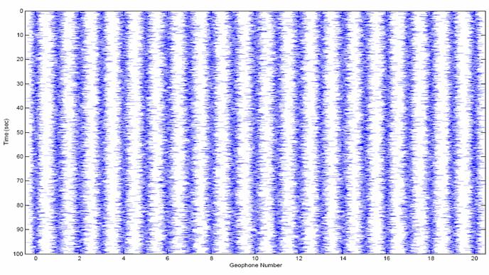
Figure 3: synthetic waveforms: random time series + reflected wavelets.

Cross-correlate the trace of S0 with each other traces in Figure 3, and the cross-correlation functions (CCFs) are plotted in the figure 4. This plotting is equivalent to a shot gather with the shot located at the station S0. The hyperbolic feature is associated with the reflector in the model. Similarly, cross-correlating each station from S1 to S20 with all other stations, the shot-gather with shot located at this station can be computed. Then the traditional techniques of reflection seismology may be applied to extract the reflectors.

Figure 4: Cross-Correlation Functions (CCFs). Cross-correlate the trace S0 with all other traces in Figure 3, respectively.